Linear Regression

Wednesday, May 27

Today we will…

• Group Quiz 8
• New Material
  • Review of Simple Linear Regression
  • Assessing Model Fit
• Work Time
  • Lab 9: Regression Exploration
  • Group Project

Project Notes

• They are coming together nicely!
• Look at Quarto documentation and the source code for our labs to see how to do quarto styling
  • links
  • callouts
  • LaTeX
  • code font (summarize())
• This is a final project – I expect clean work and evidence of effort

Simple Linear Regression

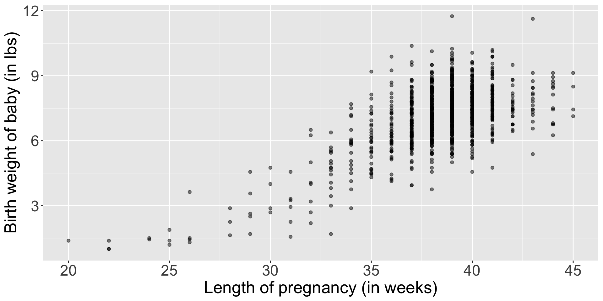
NC Births Data

This dataset contains a random sample of 1,000 births from North Carolina in 2004 (sampled from a larger dataset).

• Each case describes the birth of a single child, including characteristics of the:
  • child (birth weight, length of gestation, etc.).
  • birth parents (age, weight gained during pregnancy, smoking habits, etc.).

NC Births Data

library(openintro)
data(ncbirths)
slice_sample(ncbirths, n = 10) |> 
  knitr::kable() |> 
  kableExtra::scroll_box(height = "400px") |> 
  kableExtra::kable_styling(font_size = 30)

fage	mage	mature	weeks	premie	visits	marital	gained	weight	lowbirthweight	gender	habit	whitemom
19	15	younger mom	37	full term	11	not married	38	6.63	not low	female	nonsmoker	white
NA	28	younger mom	38	full term	10	married	70	8.19	not low	male	nonsmoker	white
55	46	mature mom	31	premie	8	married	25	4.56	low	female	nonsmoker	not white
36	37	mature mom	44	full term	10	married	25	8.94	not low	male	nonsmoker	white
NA	30	younger mom	39	full term	10	not married	38	11.75	not low	male	nonsmoker	white
26	23	younger mom	40	full term	14	married	28	8.38	not low	male	nonsmoker	white
40	34	younger mom	39	full term	15	married	20	6.38	not low	male	nonsmoker	not white
27	26	younger mom	39	full term	16	married	38	8.00	not low	female	nonsmoker	white
24	24	younger mom	38	full term	17	not married	13	6.56	not low	female	nonsmoker	not white
34	36	mature mom	37	full term	14	married	40	8.81	not low	male	nonsmoker	white

Relationships Between Variables

Relationships Between Variables

In statistical models, we generally have one variable that is the response and one or more variables that are explanatory.

• Response variable
  • Also: \(y\), dependent variable
  • This is the quantity we want to understand.

• Explanatory variable
  • Also: \(x\), independent variable, predictor
  • This is something we think might be related to the response.

Visualizing a Relationship

The scatterplot has been called the most “generally useful invention in the history of statistical graphics.”

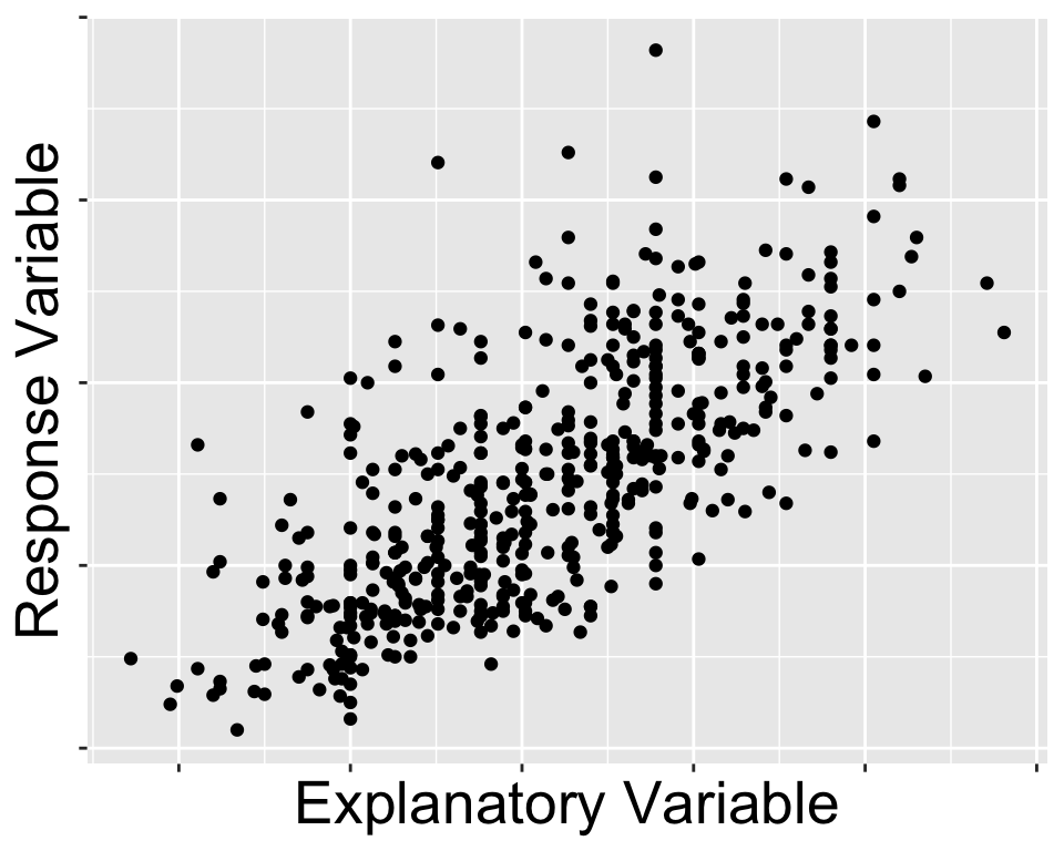
Characterizing Relationships

• Form: linear, quadratic, non-linear?
• Direction: positive, negative?
• Strength: how much scatter/noise?
• Unusual observations: do points not fit the overall pattern?

Your turn!

How would you characterize this relationship?

• Shape?
• Direction?
• Strength?
• Outliers?

Note: Much of what we are doing at this stage involves making judgment calls!

As we work through these, please keep in mind that much of what we are doing at this stage involves making judgment calls. This is part of the nature of statistics, and while it can be frustrating - especially as a beginner - it is inescapable. For better or for worse, statistics is not a field where there is one right answer. There are of course an infinite number of indefensible claims, but many judgments are open to interpretation.

There isn’t a universal, hard-and-fast definition of what constitutes an outlier, but they are often easy to spot in a scatterplot.

• What observations would you consider to be outliers?
• How would you go about removing these outliers from the data?

Fitting a Model

We often assume the value of our response variable is some function of our explanatory variable, plus some random noise.

\[response = f(explanatory) + noise\]

• There is a mathematical function \(f\) that can translate values of one variable into values of another.
• But there is some randomness in the process.

Simple Linear Regression (SLR)

If we assume the relationship between \(x\) and \(y\) takes the form of a linear function…

\[ response = intercept + slope \times explanatory + noise \]

We use the following notation for this model:

Population Regression Model

\(Y_i = \beta_0 + \beta_1 X_i + \varepsilon_i\)

where \(\varepsilon \sim N(0, \sigma)\) is the random noise.

Fitted Regression Model

\(\hat{y}_i = \hat{\beta}_0 + \hat{\beta}_1 x_i\)

where   \(\hat{}\)   indicates the value was estimated.

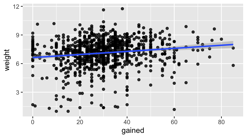
Fitting an SLR Model

• Question
• geom_smooth
• lm

Regress baby birthweight (response variable) on the pregnant parent’s weight gain (explanatory variable).

• We are assuming there is a linear relationship between how much weight the parent gains and how much the baby weighs at birth.

When visualizing data, fit a regression line (\(y\) on \(x\)) to your scatterplot.

ncbirths |> 
  ggplot(aes(x = gained, y = weight)) +
  geom_point(alpha = .8) +
  geom_smooth(method = "lm") 

The lm() function fits a linear regression model.

• We use formula notation to specify the response variable (LHS) and the explanatory variable (RHS) y ~ x.
• This code creates an lm object.

ncbirth_lm <- lm(weight ~ gained, 
                 data = ncbirths)

Model Outputs

• lm object
• Coefficients broom
• Residuals

summary(ncbirth_lm)

Call:
lm(formula = weight ~ gained, data = ncbirths)

Residuals:
    Min      1Q  Median      3Q     Max 
-6.4085 -0.6950  0.1643  0.9222  4.5158 

Coefficients:
            Estimate Std. Error t value Pr(>|t|)    
(Intercept)  6.63003    0.11120  59.620  < 2e-16 ***
gained       0.01614    0.00332   4.862 1.35e-06 ***
---
Signif. codes:  0 '***' 0.001 '**' 0.01 '*' 0.05 '.' 0.1 ' ' 1

Residual standard error: 1.474 on 971 degrees of freedom
  (27 observations deleted due to missingness)
Multiple R-squared:  0.02377,   Adjusted R-squared:  0.02276 
F-statistic: 23.64 on 1 and 971 DF,  p-value: 1.353e-06

broom::tidy(ncbirth_lm)

term	estimate	std.error	statistic	p.value
(Intercept)	6.6300336	0.1112054	59.619718	0.0e+00
gained	0.0161405	0.0033195	4.862253	1.4e-06

• Intercept: expected mean of \(y\), when \(x\) is 0.
  • Someone gaining 0 lb, will have a baby weighing 6.63 lbs, on average.

• Slope: expected change in the mean of \(y\), when \(x\) increases by 1 unit.
  • For each pound gained, the baby will weigh 0.016 lbs more, on average.

The difference between observed (point) and expected (line).

ncbirth_lm$residuals |> 
  head(3)

         1          2          3 
 0.3866279  0.9271567 -0.6133721 

resid(ncbirth_lm) |> 
  head(3)

         1          2          3 
 0.3866279  0.9271567 -0.6133721 

broom::augment(ncbirth_lm) |> 
  head(3)

.rownames	weight	gained	.fitted	.resid	.hat	.sigma	.cooksd	.std.resid
1	7.63	38	7.243372	0.3866279	0.0013265	1.474586	0.0000458	0.2624942
2	7.88	20	6.952843	0.9271567	0.0015686	1.474337	0.0003113	0.6295530
3	6.63	38	7.243372	-0.6133721	0.0013265	1.474506	0.0001152	-0.4164381

Diagnostics

Model Diagnostics

There are four conditions that must be met for a linear regression model to be appropriate:

1. Linear relationship.
2. Independent observations.
3. Normally distributed residuals.
4. Equal variance of residuals.

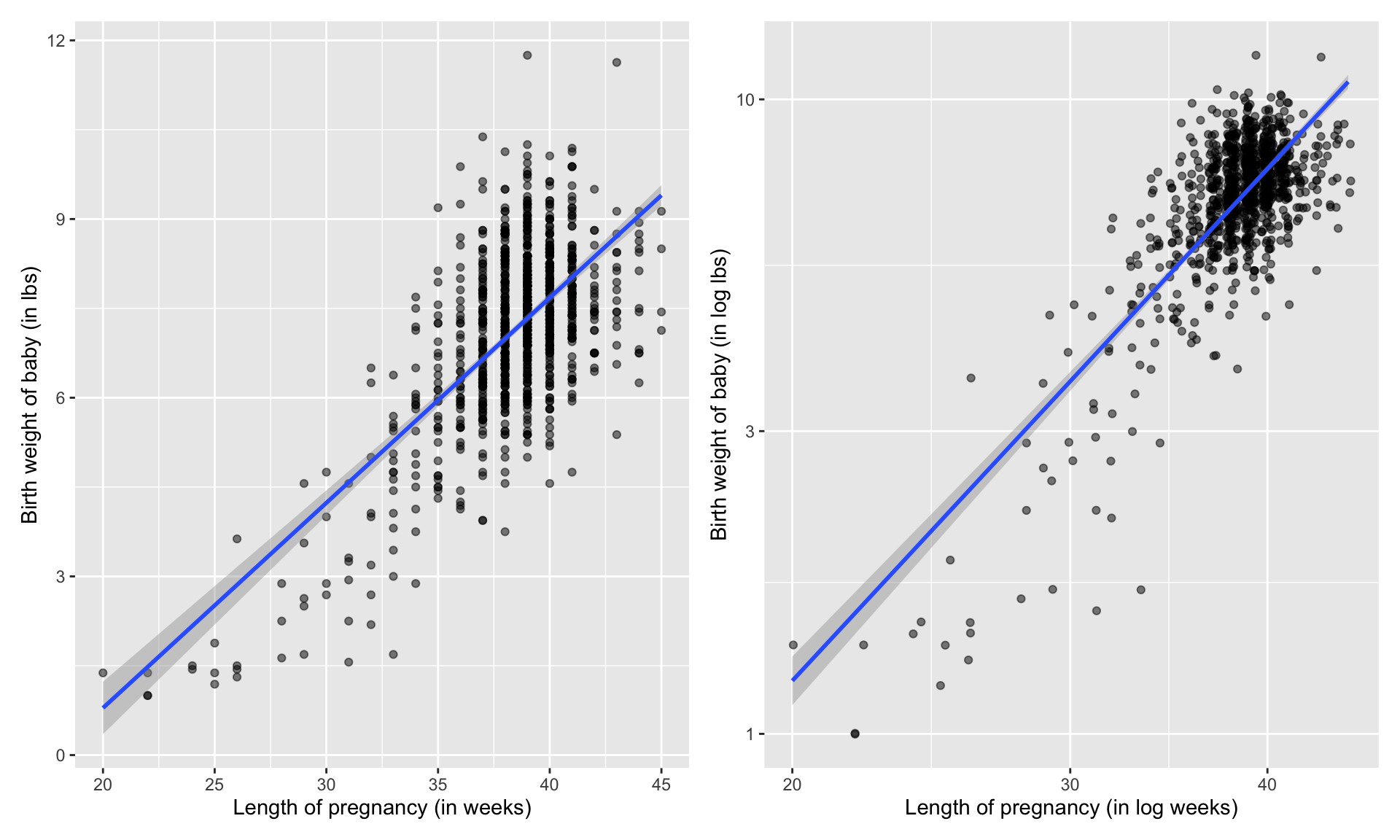
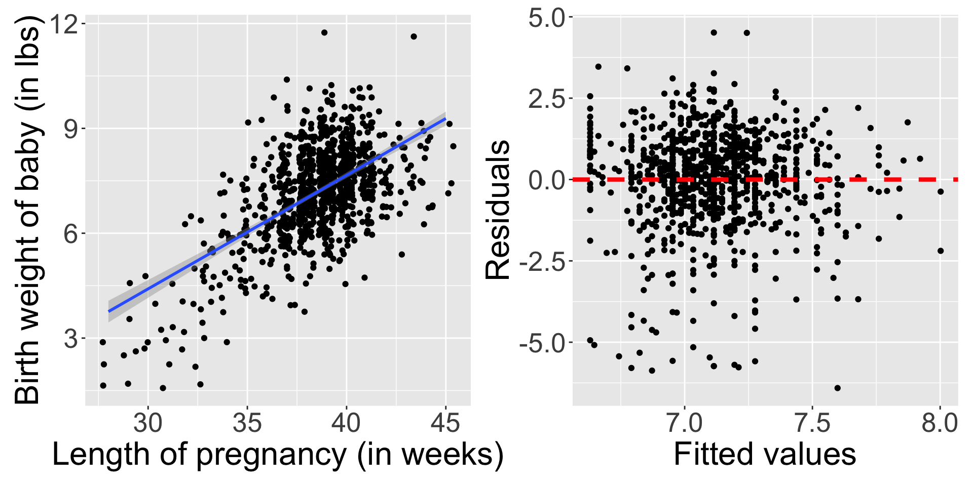
Model Diagnostics

• Linearity
• Independence
• Normality
• Equal Variance

Is the relationship linear?

• Almost nothing will look perfectly linear.
• Be careful with relationships that have curvature.
• Try transforming your variables!

Are the observations independent?   Difficult to tell!

What does independence mean?

Should not be able to know the \(y\) value for one observation based on the \(y\) value for another observation.

Independence violations:

• Stock market prices over time.
• Geographical similarities.
• Biological conditions of family members.
• Repeated observations.

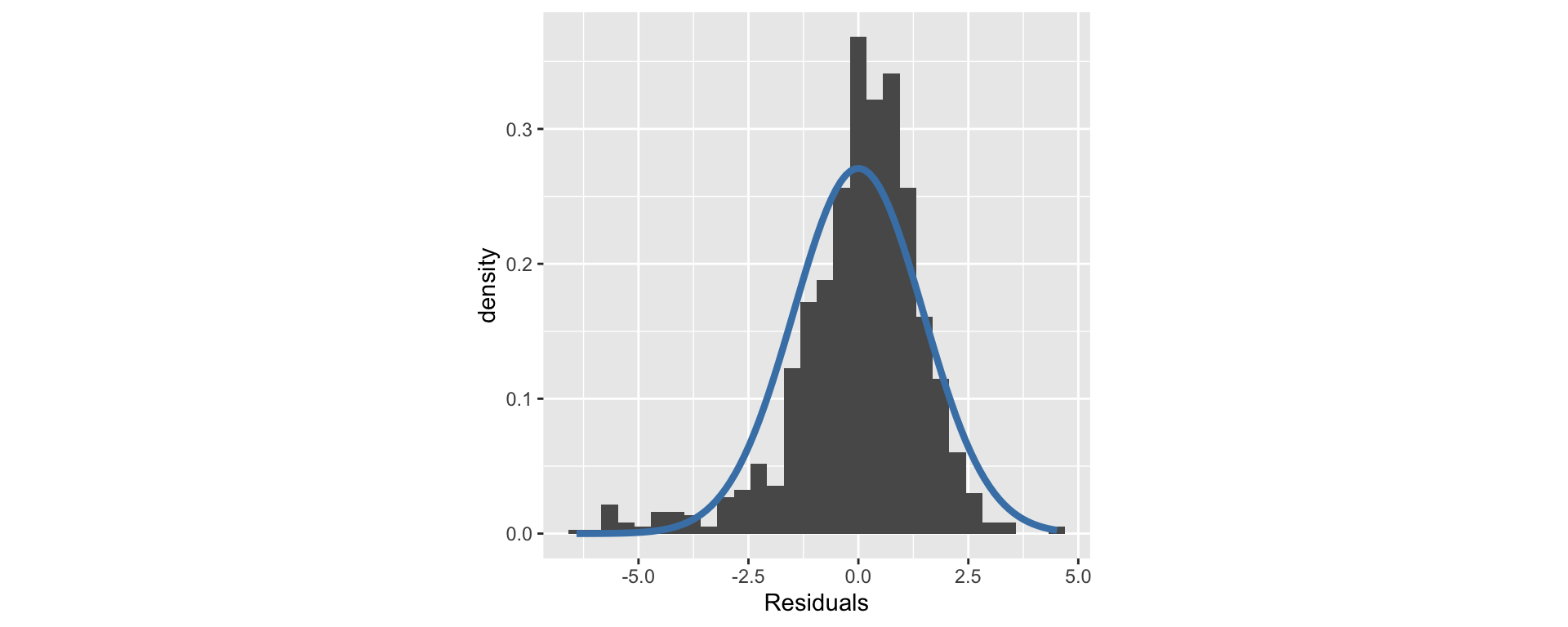
Are the residuals normally distributed?

Less important than linearity or independence:

resid_sd <- sd(ncbirth_lm$residuals)
  
ncbirth_lm |> 
  broom::augment() |> 
  ggplot(aes(x = .resid)) +
  geom_histogram(aes(y = ..density..)) +
  stat_function(fun = ~ dnorm(.x, mean = 0, sd = resid_sd),
                color = "steelblue", lwd = 1.5) +
  xlab("Residuals") +
  theme(aspect.ratio = 1)

Do the residuals have equal (constant) variance?

• The variability of points around the regression line is roughly constant.
• Data with non-equal variance across the range of \(x\) can seriously mis-estimate the variability of the slope.

ncbirth_lm |> 
  augment() |> 
  ggplot(aes(x = .fitted, y = .resid)) +
  geom_point() +
  geom_hline(yintercept = 0, linetype = "dashed", 
             color = "red", lwd = 1.5)

Assessing Model Fit

Sum of Square Errors (SSE)

• This is calculated as the sum of the squared residuals.
• A small SSE means small differences between observed and fitted values.
• Also: Sum Sq of Residuals or deviance.

Assessing Model Fit

Root Mean Square Error (RMSE)

• The standard deviation of the residuals.
• A small RMSE means small differences between observed and fitted values.
• Also: Residual standard error or sigma.

summary(ncbirth_lm)

Call:
lm(formula = weight ~ gained, data = ncbirths)

Residuals:
    Min      1Q  Median      3Q     Max 
-6.4085 -0.6950  0.1643  0.9222  4.5158 

Coefficients:
            Estimate Std. Error t value Pr(>|t|)    
(Intercept)  6.63003    0.11120  59.620  < 2e-16 ***
gained       0.01614    0.00332   4.862 1.35e-06 ***
---
Signif. codes:  0 '***' 0.001 '**' 0.01 '*' 0.05 '.' 0.1 ' ' 1

Residual standard error: 1.474 on 971 degrees of freedom
  (27 observations deleted due to missingness)
Multiple R-squared:  0.02377,   Adjusted R-squared:  0.02276 
F-statistic: 23.64 on 1 and 971 DF,  p-value: 1.353e-06

Assessing Model Fit

R-squared

• The proportion of variability in response accounted for by the linear model.
• A large R-squared means the explanatory variable is good at explaining the response.
• R-squared is between 0 and 1.

broom::glance(ncbirth_lm) |> 
  knitr::kable()

r.squared	adj.r.squared	sigma	statistic	p.value	df	logLik	AIC	BIC	deviance	df.residual	nobs
0.0237689	0.0227635	1.473879	23.6415	1.4e-06	1	-1757.05	3520.101	3534.742	2109.321	971	973

Model Comparison

Regress baby birthweight on…

… gestation weeks.

weight_weeks <- lm(weight ~ weeks, 
                   data = ncbirths)

• SSE = 1246.55
• RMSE = 1.119
• \(R^2\) = 0.449

… number of doctor visits.

weight_visits <- lm(weight ~ visits, 
                    data = ncbirths)

• SSE = 2152.74
• RMSE = 1.475
• \(R^2\) = 0.01819

Why does it make sense that the left model is better?

Multiple Linear Regression

When fitting a linear regression, you can include…

…multiple explanatory variables.

lm(y ~ x1 + x2 + x3 + ... + xn)

…interaction terms.

lm(y ~ x1 + x2 + x1:x2)

lm(y ~ x1*x2)

…quadratic relationships.

lm(y ~ I(x1^2) + x1)

Communicating Regression Model Results

• You can report the estimated linear model:

\[\hat{y}_i = 6.6 + .016x_i\]

where \(\hat{y}_i\) is the estimated birth weight in pounds and \(x_i\) is the weight gained during pregnancy by the birthing parent in pounds.

• Discuss the slope:
  • Think about units that are helpful for interpretation!
  • e.g.: We estimate that for every 10 pounds gained during pregnancy by the birthing parent the baby will weigh around 2.5 ounces more, on average.

Regression Table

• Commonly researchers will include a table like this to report the estimated coefficients and inference:

ncbirth_lm |> 
  tbl_regression(intercept = TRUE)

Characteristic	Beta	95% CI	p-value
(Intercept)	6.6	6.4, 6.8	<0.001
gained	0.02	0.01, 0.02	<0.001
Abbreviation: CI = Confidence Interval

• This is a nice build-it function from an extension of the gt package (gtsummary)

Putting it together: Fitting SLR On Subsets

The map2() Family

These functions allow us to iterate over two lists at the same time.

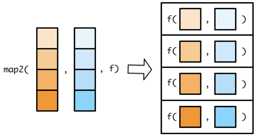
Each function has two list arguments, denoted .x and .y, and a function argument.

Small map2() Example

Find the minimum.

a <- c(1, 2, 4)
b <- c(6, 5, 3)

map2_chr(.x = a, 
         .y = b,
         ~ str_glue("The minimum of {.x} and {.y} is {min(.x, .y)}."))

[1] "The minimum of 1 and 6 is 1." "The minimum of 2 and 5 is 2."
[3] "The minimum of 4 and 3 is 3."

nest() and unnest()

• We can pair functions from the map() family very nicely with two tidyr functions: nest() and unnest().
• These allow us to easily map functions onto subsets of the data.

nest()

Nest subsets the data (as tibbles) inside a tibble.

• Specify the column(s) to create subsets on.

ncbirths |> 
  nest(premie_dat = -premie)

# A tibble: 3 × 2
  premie    premie_dat         
  <fct>     <list>             
1 full term <tibble [846 × 12]>
2 premie    <tibble [152 × 12]>
3 <NA>      <tibble [2 × 12]>  

ncbirths |> 
  nest(ph_dat = -c(premie, habit))

# A tibble: 6 × 3
  premie    habit     ph_dat             
  <fct>     <fct>     <list>             
1 full term nonsmoker <tibble [739 × 11]>
2 premie    nonsmoker <tibble [133 × 11]>
3 full term smoker    <tibble [107 × 11]>
4 premie    smoker    <tibble [19 × 11]> 
5 <NA>      nonsmoker <tibble [1 × 11]>  
6 <NA>      <NA>      <tibble [1 × 11]>  

unnest()

Un-nest the data by row binding the subsets back together.

• Specify the column(s) that contains the subsets.

ncbirths |> 
  nest(premie_dat = -premie) |> 
  unnest(premie_dat) |> 
  head()

# A tibble: 6 × 13
  premie     fage  mage mature weeks visits marital gained weight lowbirthweight
  <fct>     <int> <int> <fct>  <int>  <int> <fct>    <int>  <dbl> <fct>         
1 full term    NA    13 young…    39     10 not ma…     38   7.63 not low       
2 full term    NA    14 young…    42     15 not ma…     20   7.88 not low       
3 full term    19    15 young…    37     11 not ma…     38   6.63 not low       
4 full term    21    15 young…    41      6 not ma…     34   8    not low       
5 full term    NA    15 young…    39      9 not ma…     27   6.38 not low       
6 full term    NA    15 young…    38     19 not ma…     22   5.38 low           
# ℹ 3 more variables: gender <fct>, habit <fct>, whitemom <fct>

Big map2() Example - Regression

• nest()
• lm()
• predict()
• unnest()

ncbirths_clean <- ncbirths |> 
    filter(!if_any(.cols = c(premie, habit, weight, gained),
                 .fns = is.na))

ncbirths_clean |> 
  nest(ph_dat = -c(premie, habit))

# A tibble: 4 × 3
  premie    habit     ph_dat             
  <fct>     <fct>     <list>             
1 full term nonsmoker <tibble [724 × 11]>
2 premie    nonsmoker <tibble [126 × 11]>
3 full term smoker    <tibble [103 × 11]>
4 premie    smoker    <tibble [19 × 11]> 

ncbirths_clean |> 
  nest(premie_smoke_dat = -c(premie, habit)) |> 
  mutate(mod = map(premie_smoke_dat, 
                   ~ lm(weight ~ gained, data = .x)))

# A tibble: 4 × 4
  premie    habit     premie_smoke_dat    mod   
  <fct>     <fct>     <list>              <list>
1 full term nonsmoker <tibble [724 × 11]> <lm>  
2 premie    nonsmoker <tibble [126 × 11]> <lm>  
3 full term smoker    <tibble [103 × 11]> <lm>  
4 premie    smoker    <tibble [19 × 11]>  <lm>  

ncbirths_clean |> 
  nest(premie_smoke_dat = -c(premie, habit)) |> 
  mutate(mod = map(premie_smoke_dat, 
                   ~ lm(weight ~ gained, data = .x)),
         pred_weight = map2(.x = mod,
                         .y = premie_smoke_dat, 
                         .f = ~ predict(object = .x, data = .y)))

# A tibble: 4 × 5
  premie    habit     premie_smoke_dat    mod    pred_weight
  <fct>     <fct>     <list>              <list> <list>     
1 full term nonsmoker <tibble [724 × 11]> <lm>   <dbl [724]>
2 premie    nonsmoker <tibble [126 × 11]> <lm>   <dbl [126]>
3 full term smoker    <tibble [103 × 11]> <lm>   <dbl [103]>
4 premie    smoker    <tibble [19 × 11]>  <lm>   <dbl [19]> 

ncbirths_clean |> 
  nest(premie_smoke_dat = -c(premie, habit)) |> 
  mutate(mod = map(premie_smoke_dat, 
                   ~ lm(weight ~ gained, data = .x)),
         pred_weight = map2(.x = mod,
                         .y = premie_smoke_dat, 
                         .f = ~ predict(object = .x, data = .y))) |> 
  select(-mod) |> 
  unnest(cols = c(premie_smoke_dat, pred_weight)) |> 
  select(premie, habit, weight, gained, pred_weight) |> 
  head()

# A tibble: 6 × 5
  premie    habit     weight gained pred_weight
  <fct>     <fct>      <dbl>  <int>       <dbl>
1 full term nonsmoker   7.63     38        7.55
2 full term nonsmoker   7.88     20        7.43
3 full term nonsmoker   6.63     38        7.55
4 full term nonsmoker   8        34        7.53
5 full term nonsmoker   6.38     27        7.48
6 full term nonsmoker   5.38     22        7.44

Example Cont. - Regression Coefficients

• nest() + lm()
• Pull Coefficients
• Format Table

ncbirths_clean |> 
  nest(premie_smoke_dat = -c(premie, habit)) |> 
  mutate(mod = map(premie_smoke_dat, 
                   ~ lm(weight ~ gained, data = .x)),
         coefs = map(mod,
                      ~ broom::tidy(.x))) 

# A tibble: 4 × 5
  premie    habit     premie_smoke_dat    mod    coefs           
  <fct>     <fct>     <list>              <list> <list>          
1 full term nonsmoker <tibble [724 × 11]> <lm>   <tibble [2 × 5]>
2 premie    nonsmoker <tibble [126 × 11]> <lm>   <tibble [2 × 5]>
3 full term smoker    <tibble [103 × 11]> <lm>   <tibble [2 × 5]>
4 premie    smoker    <tibble [19 × 11]>  <lm>   <tibble [2 × 5]>

ncbirths_clean |> 
  nest(premie_smoke_dat = -c(premie, habit)) |> 
  mutate(mod = map(premie_smoke_dat, 
                   ~ lm(weight ~ gained, data = .x)),
         coefs = map(mod,
                      ~ broom::tidy(.x))) |> 
  select(premie, habit, coefs) |> 
  unnest(cols = coefs)

# A tibble: 8 × 7
  premie    habit     term        estimate std.error statistic  p.value
  <fct>     <fct>     <chr>          <dbl>     <dbl>     <dbl>    <dbl>
1 full term nonsmoker (Intercept)  7.29      0.0965      75.5  0       
2 full term nonsmoker gained       0.00705   0.00285      2.48 1.34e- 2
3 premie    nonsmoker (Intercept)  4.55      0.393       11.6  1.75e-21
4 premie    nonsmoker gained       0.0258    0.0137       1.89 6.09e- 2
5 full term smoker    (Intercept)  6.77      0.223       30.3  1.71e-52
6 full term smoker    gained       0.0121    0.00613      1.98 5.08e- 2
7 premie    smoker    (Intercept)  5.75      0.880        6.54 5.04e- 6
8 premie    smoker    gained      -0.0320    0.0293      -1.09 2.89e- 1

ncbirths_clean |> 
  nest(premie_smoke_dat = -c(premie, habit)) |> 
  mutate(mod = map(premie_smoke_dat, 
                   ~ lm(weight ~ gained, data = .x)),
         coefs = map(mod,
                      ~ broom::tidy(.x))) |> 
  select(premie, habit, coefs) |> 
  unnest(cols = coefs) |> 
  mutate(term = fct_recode(.f = term,
                            "Intercept" = "(Intercept)",
                            "Mother Weight Gain (lb.)" = "gained"
                            )) |> 
  select(-std.error, -statistic) |> 
  mutate(p.value = case_when(p.value < .0001 ~ "<.001",
                             TRUE ~ as.character(round(p.value, 3)))) |> 
  arrange(premie, habit, term) |> 
  gt() |> 
  fmt_number(estimate,
             decimals = 3) |> 
  tab_row_group(
    label = md("**Premature + Smoker**"),
    rows = premie == "premie" & habit == "smoker") |> 
  tab_row_group(
    label = md("**Premature + Non-Smoker**"),
    rows = premie == "premie" & habit == "nonsmoker") |> 
  tab_row_group(
    label = md("**Full Term + Smoker**"),
    rows = premie == "full term" & habit == "smoker") |> 
  tab_row_group(
    label = md("**Full Term + Non-Smoker**"),
    rows = premie == "full term" & habit == "nonsmoker") |> 
  cols_hide(c(premie, habit)) |> 
  cols_align(align = "left",
             columns = term) |> 
  tab_style(
    style = cell_fill(color = "gray85"),
    locations = cells_row_groups()) |> 
  cols_label(
    "term" = md("**Model & Term**"),
    "estimate" = md("**Est. Coef.**"),
    "p.value" = md("**p-value**")
  ) 

Model & Term	Est. Coef.	p-value
Full Term + Non-Smoker
Intercept	7.285	<.001
Mother Weight Gain (lb.)	0.007	0.013
Full Term + Smoker
Intercept	6.767	<.001
Mother Weight Gain (lb.)	0.012	0.051
Premature + Non-Smoker
Intercept	4.549	<.001
Mother Weight Gain (lb.)	0.026	0.061
Premature + Smoker
Intercept	5.754	<.001
Mother Weight Gain (lb.)	−0.032	0.289

Lab 9: Regression Exploration

To do…

• Optional Project Checkpoint 4
  • Due Friday 5/29 at 11:59pm.
• Lab 9: Simulation Exploration
  • Due Tuesday 6/2 at 11:59pm.
• Required Reading
  • Review the material from this week for the final Group Quiz Monday