Week 4, Part 1: Data Joins and Pivots
1 Learning Objectives
- Determine what data format is necessary to generate a desired plot or statistical model.
- Understand the differences between “wide” and “long” format data and how to transition between the two structures.
- Understand relational data formats and how to use data joins to assemble data from multiple tables into a single table.
📖 Readings: 75 min
📽 Optional Videos: 25 min
2 Relational Data and Joins
📖 Required Reading: R4DS 19.1-19.4: Joins
- Note: don’t read 19.5! We will not cover non-equi joins in this course
3 Data Transformation
Data Pivots
📖 Required Reading: R4DS 5: Data tidying
📽 Optional Videos
Splitting Cells
Expanding on what we talked about in class, there’s a task that is fairly commonly encountered with functions that belong to the tidyr package: separating variables into two different columns separate_xxx() and it’s complement, unite(), which is useful for combining two variables into one column.
The datasets used in the examples below are included in the tidyr package!
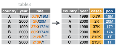
Table 3 from before is a great example of when you would want to separate the values of a column into different columns. In this dataset, the variable rate is recorded as 745/19987071, where the first number is the amount of cases and the second number is the population.
table3 |>
kable()| country | year | rate |
|---|---|---|
| Afghanistan | 1999 | 745/19987071 |
| Afghanistan | 2000 | 2666/20595360 |
| Brazil | 1999 | 37737/172006362 |
| Brazil | 2000 | 80488/174504898 |
| China | 1999 | 212258/1272915272 |
| China | 2000 | 213766/1280428583 |
table3 |>
  separate_wider_delim(cols        = rate,
                       names       = c("cases", "population"),
                       delim       = "/",
                       cols_remove = FALSE
           ) |>
kable()| country | year | cases | population | rate |
|---|---|---|---|---|
| Afghanistan | 1999 | 745 | 19987071 | 745/19987071 |
| Afghanistan | 2000 | 2666 | 20595360 | 2666/20595360 |
| Brazil | 1999 | 37737 | 172006362 | 37737/172006362 |
| Brazil | 2000 | 80488 | 174504898 | 80488/174504898 |
| China | 1999 | 212258 | 1272915272 | 212258/1272915272 |
| China | 2000 | 213766 | 1280428583 | 213766/1280428583 |
I’ve left the rate column in the original data frame (cols_remove = FALSE) just to make it easy to compare and verify that yes, it worked.
And, of course, there is a complementary operation, which is when it’s necessary to join two columns to get a useable data value.
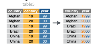
table5 |>
kable()| country | century | year | rate |
|---|---|---|---|
| Afghanistan | 19 | 99 | 745/19987071 |
| Afghanistan | 20 | 00 | 2666/20595360 |
| Brazil | 19 | 99 | 37737/172006362 |
| Brazil | 20 | 00 | 80488/174504898 |
| China | 19 | 99 | 212258/1272915272 |
| China | 20 | 00 | 213766/1280428583 |
table5 |>
  unite(col = "year",
        c(century, year),
        sep = ''
        ) |>
kable()| country | year | rate |
|---|---|---|
| Afghanistan | 1999 | 745/19987071 |
| Afghanistan | 2000 | 2666/20595360 |
| Brazil | 1999 | 37737/172006362 |
| Brazil | 2000 | 80488/174504898 |
| China | 1999 | 212258/1272915272 |
| China | 2000 | 213766/1280428583 |