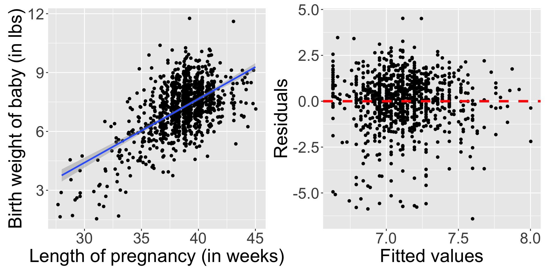
Linear Regression

Thursday, May 29

Today we will…

• Data Intro + Cleaning: Feedback
• New Material
  • Review of Simple Linear Regression
  • Assessing Model Fit
• Work Time
  • PA 9: Mystery Animal
  • PC4: Linear Regression

Data Intro + Cleaning: Feedback

General:

• Overall these are looking good!
  • Lots of interesting topics to explore.
  • Nice insights and descriptions of data sources
• Before the final submission, read all instructions carefully
  • Project Details
  • Project Report Writing Guide
  • Citations Guide

Data Intro + Cleaning: Feedback

Code:

• All code should be hidden – use echo: false or code-fold: true in your YAML.
• Don’t name the R functions you have used (“We used str_detect to…”.).
  • Instead, describe what you did in plain English.
• Don’t use dataset or variable names in the text.
  • Say “We removed missing values from per capita GDP.” rather than “We removed NA from per_cap_gdp.”
• Don’t print out the head of the data!

Data Intro + Cleaning: Feedback

Citations:

• Cite your sources, including:
  • data sources.
  • description of your variables that is not general knowledge.
  • any other outside resources.
• You should have both in-line citations and a References section at the end of your report.
  • see intstuctions on Canvas

Data Intro + Cleaning: Feedback

Style + Organization:

• Define all acronyms, especially any that are related to the variables of interest.
• Everything should be in paragraph form
  • no bullets or numbered lists unless there is a very good reason
• Read through your paper from top to bottom to make sure the organization makes sense.
  • At what point might someone get confused?

Simple Linear Regression

NC Births Data

This dataset contains a random sample of 1,000 births from North Carolina in 2004 (sampled from a larger dataset).

• Each case describes the birth of a single child, including characteristics of the:
  • child (birth weight, length of gestation, etc.).
  • birth parents (age, weight gained during pregnancy, smoking habits, etc.).

NC Births Data

library(openintro)
data(ncbirths)
slice_sample(ncbirths, n = 10) |> 
  knitr::kable() |> 
  kableExtra::scroll_box(height = "400px") |> 
  kableExtra::kable_styling(font_size = 30)

fage	mage	mature	weeks	premie	visits	marital	gained	weight	lowbirthweight	gender	habit	whitemom
37	33	younger mom	38	full term	13	married	18	8.63	not low	male	nonsmoker	white
33	28	younger mom	41	full term	10	married	30	8.13	not low	male	nonsmoker	not white
32	31	younger mom	37	full term	13	married	30	10.38	not low	male	nonsmoker	white
38	33	younger mom	39	full term	12	married	25	9.25	not low	male	nonsmoker	not white
38	33	younger mom	38	full term	14	married	30	5.88	not low	male	nonsmoker	white
25	24	younger mom	40	full term	15	married	29	8.50	not low	female	nonsmoker	white
31	26	younger mom	36	premie	18	married	40	8.00	not low	male	nonsmoker	white
33	34	younger mom	40	full term	13	married	25	8.25	not low	male	nonsmoker	white
NA	19	younger mom	39	full term	9	not married	35	7.75	not low	male	nonsmoker	not white
32	27	younger mom	43	full term	11	married	30	6.56	not low	female	nonsmoker	not white

Relationships Between Variables

Relationships Between Variables

In statistical models, we generally have one variable that is the response and one or more variables that are explanatory.

• Response variable
  • Also: \(y\), dependent variable
  • This is the quantity we want to understand.

• Explanatory variable
  • Also: \(x\), independent variable, predictor
  • This is something we think might be related to the response.

Visualizing a Relationship

The scatterplot has been called the most “generally useful invention in the history of statistical graphics.”

Characterizing Relationships

• Form: linear, quadratic, non-linear?
• Direction: positive, negative?
• Strength: how much scatter/noise?
• Unusual observations: do points not fit the overall pattern?

Your turn!

How would you characterize this relationship?

• Shape?
• Direction?
• Strength?
• Outliers?

Note: Much of what we are doing at this stage involves making judgment calls!

As we work through these, please keep in mind that much of what we are doing at this stage involves making judgment calls. This is part of the nature of statistics, and while it can be frustrating - especially as a beginner - it is inescapable. For better or for worse, statistics is not a field where there is one right answer. There are of course an infinite number of indefensible claims, but many judgments are open to interpretation.

There isn’t a universal, hard-and-fast definition of what constitutes an outlier, but they are often easy to spot in a scatterplot.

• What observations would you consider to be outliers?
• How would you go about removing these outliers from the data?

Fitting a Model

We often assume the value of our response variable is some function of our explanatory variable, plus some random noise.

\[response = f(explanatory) + noise\]

• There is a mathematical function \(f\) that can translate values of one variable into values of another.
• But there is some randomness in the process.

Simple Linear Regression (SLR)

If we assume the relationship between \(x\) and \(y\) takes the form of a linear function…

\[ response = intercept + slope \times explanatory + noise \]

We use the following notation for this model:

Population Regression Model

\(Y = \beta_0 + \beta_1 X + \varepsilon\)

where \(\varepsilon \sim N(0, \sigma)\) is the random noise.

Fitted Regression Model

\(\hat{y}_i = \hat{\beta}_0 + \hat{\beta}_1 x_i\)

where   \(\hat{}\)   indicates the value was estimated.

Fitting an SLR Model

• Question
• geom_smooth
• lm

Regress baby birthweight (response variable) on the pregnant parent’s weight gain (explanatory variable).

• We are assuming there is a linear relationship between how much weight the parent gains and how much the baby weighs at birth.

When visualizing data, fit a regression line (\(y\) on \(x\)) to your scatterplot.

ncbirths |> 
  ggplot(aes(x = gained, y = weight)) +
  geom_jitter() + 
  geom_smooth(method = "lm") 

The lm() function fits a linear regression model.

• We use formula notation to specify the response variable (LHS) and the explanatory variable (RHS).
• This code creates an lm object.

ncbirth_lm <- lm(weight ~ gained, 
                 data = ncbirths)

Model Outputs

• lm object
• Coefficients broom
• Residuals

summary(ncbirth_lm)

Call:
lm(formula = weight ~ gained, data = ncbirths)

Residuals:
    Min      1Q  Median      3Q     Max 
-6.4085 -0.6950  0.1643  0.9222  4.5158 

Coefficients:
            Estimate Std. Error t value Pr(>|t|)    
(Intercept)  6.63003    0.11120  59.620  < 2e-16 ***
gained       0.01614    0.00332   4.862 1.35e-06 ***
---
Signif. codes:  0 '***' 0.001 '**' 0.01 '*' 0.05 '.' 0.1 ' ' 1

Residual standard error: 1.474 on 971 degrees of freedom
  (27 observations deleted due to missingness)
Multiple R-squared:  0.02377,   Adjusted R-squared:  0.02276 
F-statistic: 23.64 on 1 and 971 DF,  p-value: 1.353e-06

broom::tidy(ncbirth_lm)

term	estimate	std.error	statistic	p.value
(Intercept)	6.6300336	0.1112054	59.619718	0.0e+00
gained	0.0161405	0.0033195	4.862253	1.4e-06

• Intercept: expected mean of \(y\), when \(x\) is 0.
  • Someone gaining 0 lb, will have a baby weighing 6.63 lbs, on average.

• Slope: expected change in the mean of \(y\), when \(x\) increases by 1 unit.
  • For each pound gained, the baby will weigh 0.016 lbs more, on average.

The difference between observed (point) and expected (line).

ncbirth_lm$residuals |> 
  head(3)

         1          2          3 
 0.3866279  0.9271567 -0.6133721 

resid(ncbirth_lm) |> 
  head(3)

         1          2          3 
 0.3866279  0.9271567 -0.6133721 

broom::augment(ncbirth_lm) |> 
  head(3)

.rownames	weight	gained	.fitted	.resid	.hat	.sigma	.cooksd	.std.resid
1	7.63	38	7.243372	0.3866279	0.0013265	1.474586	0.0000458	0.2624942
2	7.88	20	6.952843	0.9271567	0.0015686	1.474337	0.0003113	0.6295530
3	6.63	38	7.243372	-0.6133721	0.0013265	1.474506	0.0001152	-0.4164381

Diagnostics

Model Diagnostics

There are four conditions that must be met for a linear regression model to be appropriate:

1. Linear relationship.
2. Independent observations.
3. Normally distributed residuals.
4. Equal variance of residuals.

Model Diagnostics

• Linearity
• Independence
• Normality
• Equal Variance

Is the relationship linear?

• Almost nothing will look perfectly linear.
• Be careful with relationships that have curvature.
• Try transforming your variables!

Are the observations independent?   Difficult to tell!

What does independence mean?

Should not be able to know the \(y\) value for one observation based on the \(y\) value for another observation.

Independence violations:

• Stock market prices over time.
• Geographical similarities.
• Biological conditions of family members.
• Repeated observations.

Are the residuals normally distributed?

Less important than linearity or independence:

Do the residuals have equal (constant) variance?

• The variability of points around the regression line is roughly constant.
• Data with non-equal variance across the range of \(x\) can seriously mis-estimate the variability of the slope.

ncbirth_lm |> 
  augment() |> 
  ggplot(aes(x = .fitted, y = .resid)) +
  geom_point() +
  geom_hline(yintercept = 0, linetype = "dashed", 
             color = "red", lwd = 1.5)

Assessing Model Fit

Sum of Square Errors (SSE)

• This is calculated as the sum of the squared residuals.
• A small SSE means small differences between observed and fitted values.
• Also: Sum Sq of Residuals or deviance.

Assessing Model Fit

Root Mean Square Error (RMSE)

• The standard deviation of the residuals.
• A small RMSE means small differences between observed and fitted values.
• Also: Residual standard error or sigma.

summary(ncbirth_lm)

Call:
lm(formula = weight ~ gained, data = ncbirths)

Residuals:
    Min      1Q  Median      3Q     Max 
-6.4085 -0.6950  0.1643  0.9222  4.5158 

Coefficients:
            Estimate Std. Error t value Pr(>|t|)    
(Intercept)  6.63003    0.11120  59.620  < 2e-16 ***
gained       0.01614    0.00332   4.862 1.35e-06 ***
---
Signif. codes:  0 '***' 0.001 '**' 0.01 '*' 0.05 '.' 0.1 ' ' 1

Residual standard error: 1.474 on 971 degrees of freedom
  (27 observations deleted due to missingness)
Multiple R-squared:  0.02377,   Adjusted R-squared:  0.02276 
F-statistic: 23.64 on 1 and 971 DF,  p-value: 1.353e-06

Assessing Model Fit

R-squared

• The proportion of variability in response accounted for by the linear model.
• A large R-squared means the explanatory variable is good at explaining the response.
• R-squared is between 0 and 1.

broom::glance(ncbirth_lm) |> 
  knitr::kable()

r.squared	adj.r.squared	sigma	statistic	p.value	df	logLik	AIC	BIC	deviance	df.residual	nobs
0.0237689	0.0227635	1.473879	23.6415	1.4e-06	1	-1757.05	3520.101	3534.742	2109.321	971	973

Model Comparison

Regress baby birthweight on…

… gestation weeks.

weight_weeks <- lm(weight ~ weeks, 
                   data = ncbirths)

• SSE = 1246.55
• RMSE = 1.119
• \(R^2\) = 0.449

… number of doctor visits.

weight_visits <- lm(weight ~ visits, 
                    data = ncbirths)

• SSE = 2152.74
• RMSE = 1.475
• \(R^2\) = 0.01819

Why does it make sense that the left model is better?

Multiple Linear Regression

When fitting a linear regression, you can include…

…multiple explanatory variables.

lm(y ~ x1 + x2 + x3 + ... + xn)

…interaction terms.

lm(y ~ x1 + x2 + x1:x2)

lm(y ~ x1*x2)

…quadratic relationships.

lm(y ~ I(x1^2) + x1)

Communicating Regression Model Results

• You can report the estimated linear model:

\[\hat{y}_i = 6.6 + .016x_i\]

where \(\hat{y}_i\) is the estimated birth weight in pounds and \(x_i\) is the weight gained during pregnancy by the birthing parent in pounds.

• Discuss the slope:
  • Think about units that are helpful for interpretation!
  • e.g.: We estimate that for every 10 pounds gained during pregnancy by the birthing parent the baby will weigh around 2.5 ounces more, on average.

Regression Table

• Commonly researchers will include a table like this to report the estimated coefficients and inference:

ncbirth_lm |> 
  tbl_regression(intercept = TRUE)

Characteristic	Beta	95% CI	p-value
(Intercept)	6.6	6.4, 6.8	<0.001
gained	0.02	0.01, 0.02	<0.001
Abbreviation: CI = Confidence Interval

• This is a nice build-it function from an extension of the gt package (gtsummary)

Putting it together: Fitting SLR On Subsets

The map2() Family

These functions allow us to iterate over two lists at the same time.

Each function has two list arguments, denoted .x and .y, and a function argument.

Small map2() Example

Find the minimum.

a <- c(1, 2, 4)
b <- c(6, 5, 3)

map2_chr(.x = a, 
         .y = b,
         ~ str_glue("The minimum of {.x} and {.y} is {min(.x, .y)}."))

[1] "The minimum of 1 and 6 is 1." "The minimum of 2 and 5 is 2."
[3] "The minimum of 4 and 3 is 3."

nest() and unnest()

• We can pair functions from the map() family very nicely with two tidyr functions: nest() and unnest().
• These allow us to easily map functions onto subsets of the data.

nest()

Nest subsets the data (as tibbles) inside a tibble.

• Specify the column(s) to create subsets on.

ncbirths |> 
  nest(premie_dat = -premie)

# A tibble: 3 × 2
  premie    premie_dat         
  <fct>     <list>             
1 full term <tibble [846 × 12]>
2 premie    <tibble [152 × 12]>
3 <NA>      <tibble [2 × 12]>  

ncbirths |> 
  nest(ph_dat = -c(premie, habit))

# A tibble: 6 × 3
  premie    habit     ph_dat             
  <fct>     <fct>     <list>             
1 full term nonsmoker <tibble [739 × 11]>
2 premie    nonsmoker <tibble [133 × 11]>
3 full term smoker    <tibble [107 × 11]>
4 premie    smoker    <tibble [19 × 11]> 
5 <NA>      nonsmoker <tibble [1 × 11]>  
6 <NA>      <NA>      <tibble [1 × 11]>  

unnest()

Un-nest the data by row binding the subsets back together.

• Specify the column(s) that contains the subsets.

ncbirths |> 
  nest(premie_dat = -premie) |> 
  unnest(premie_dat) |> 
  head()

# A tibble: 6 × 13
  premie     fage  mage mature weeks visits marital gained weight lowbirthweight
  <fct>     <int> <int> <fct>  <int>  <int> <fct>    <int>  <dbl> <fct>         
1 full term    NA    13 young…    39     10 not ma…     38   7.63 not low       
2 full term    NA    14 young…    42     15 not ma…     20   7.88 not low       
3 full term    19    15 young…    37     11 not ma…     38   6.63 not low       
4 full term    21    15 young…    41      6 not ma…     34   8    not low       
5 full term    NA    15 young…    39      9 not ma…     27   6.38 not low       
6 full term    NA    15 young…    38     19 not ma…     22   5.38 low           
# ℹ 3 more variables: gender <fct>, habit <fct>, whitemom <fct>

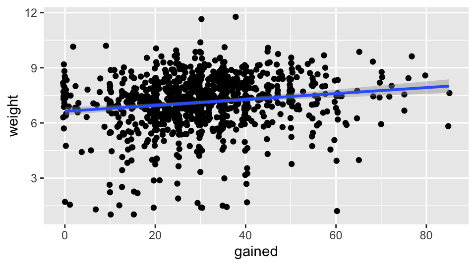
Big map2() Example - Regression

• nest()
• lm()
• predict()
• unnest()

ncbirths_clean <- ncbirths |> 
    filter(!if_any(.cols = c(premie, habit, weight, gained),
                 .fns = is.na))

ncbirths_clean |> 
  nest(ph_dat = -c(premie, habit))

# A tibble: 4 × 3
  premie    habit     ph_dat             
  <fct>     <fct>     <list>             
1 full term nonsmoker <tibble [724 × 11]>
2 premie    nonsmoker <tibble [126 × 11]>
3 full term smoker    <tibble [103 × 11]>
4 premie    smoker    <tibble [19 × 11]> 

ncbirths_clean |> 
  nest(premie_smoke_dat = -c(premie, habit)) |> 
  mutate(mod = map(premie_smoke_dat, 
                   ~ lm(weight ~ gained, data = .x)))

# A tibble: 4 × 4
  premie    habit     premie_smoke_dat    mod   
  <fct>     <fct>     <list>              <list>
1 full term nonsmoker <tibble [724 × 11]> <lm>  
2 premie    nonsmoker <tibble [126 × 11]> <lm>  
3 full term smoker    <tibble [103 × 11]> <lm>  
4 premie    smoker    <tibble [19 × 11]>  <lm>  

ncbirths_clean |> 
  nest(premie_smoke_dat = -c(premie, habit)) |> 
  mutate(mod = map(premie_smoke_dat, 
                   ~ lm(weight ~ gained, data = .x)),
         pred_weight = map2(.x = mod,
                         .y = premie_smoke_dat, 
                         .f = ~ predict(object = .x, data = .y)))

# A tibble: 4 × 5
  premie    habit     premie_smoke_dat    mod    pred_weight
  <fct>     <fct>     <list>              <list> <list>     
1 full term nonsmoker <tibble [724 × 11]> <lm>   <dbl [724]>
2 premie    nonsmoker <tibble [126 × 11]> <lm>   <dbl [126]>
3 full term smoker    <tibble [103 × 11]> <lm>   <dbl [103]>
4 premie    smoker    <tibble [19 × 11]>  <lm>   <dbl [19]> 

ncbirths_clean |> 
  nest(premie_smoke_dat = -c(premie, habit)) |> 
  mutate(mod = map(premie_smoke_dat, 
                   ~ lm(weight ~ gained, data = .x)),
         pred_weight = map2(.x = mod,
                         .y = premie_smoke_dat, 
                         .f = ~ predict(object = .x, data = .y))) |> 
  select(-mod) |> 
  unnest(cols = c(premie_smoke_dat, pred_weight)) |> 
  select(premie, habit, weight, gained, pred_weight) |> 
  head()

# A tibble: 6 × 5
  premie    habit     weight gained pred_weight
  <fct>     <fct>      <dbl>  <int>       <dbl>
1 full term nonsmoker   7.63     38        7.55
2 full term nonsmoker   7.88     20        7.43
3 full term nonsmoker   6.63     38        7.55
4 full term nonsmoker   8        34        7.53
5 full term nonsmoker   6.38     27        7.48
6 full term nonsmoker   5.38     22        7.44

Example Cont. - Regression Coefficients

• nest() + lm()
• Pull Coefficients
• Format Table

ncbirths_clean |> 
  nest(premie_smoke_dat = -c(premie, habit)) |> 
  mutate(mod = map(premie_smoke_dat, 
                   ~ lm(weight ~ gained, data = .x)),
         coefs = map(mod,
                      ~ broom::tidy(.x))) 

# A tibble: 4 × 5
  premie    habit     premie_smoke_dat    mod    coefs           
  <fct>     <fct>     <list>              <list> <list>          
1 full term nonsmoker <tibble [724 × 11]> <lm>   <tibble [2 × 5]>
2 premie    nonsmoker <tibble [126 × 11]> <lm>   <tibble [2 × 5]>
3 full term smoker    <tibble [103 × 11]> <lm>   <tibble [2 × 5]>
4 premie    smoker    <tibble [19 × 11]>  <lm>   <tibble [2 × 5]>

ncbirths_clean |> 
  nest(premie_smoke_dat = -c(premie, habit)) |> 
  mutate(mod = map(premie_smoke_dat, 
                   ~ lm(weight ~ gained, data = .x)),
         coefs = map(mod,
                      ~ broom::tidy(.x))) |> 
  select(premie, habit, coefs) |> 
  unnest(cols = coefs)

# A tibble: 8 × 7
  premie    habit     term        estimate std.error statistic  p.value
  <fct>     <fct>     <chr>          <dbl>     <dbl>     <dbl>    <dbl>
1 full term nonsmoker (Intercept)  7.29      0.0965      75.5  0       
2 full term nonsmoker gained       0.00705   0.00285      2.48 1.34e- 2
3 premie    nonsmoker (Intercept)  4.55      0.393       11.6  1.75e-21
4 premie    nonsmoker gained       0.0258    0.0137       1.89 6.09e- 2
5 full term smoker    (Intercept)  6.77      0.223       30.3  1.71e-52
6 full term smoker    gained       0.0121    0.00613      1.98 5.08e- 2
7 premie    smoker    (Intercept)  5.75      0.880        6.54 5.04e- 6
8 premie    smoker    gained      -0.0320    0.0293      -1.09 2.89e- 1

ncbirths_clean |> 
  nest(premie_smoke_dat = -c(premie, habit)) |> 
  mutate(mod = map(premie_smoke_dat, 
                   ~ lm(weight ~ gained, data = .x)),
         coefs = map(mod,
                      ~ broom::tidy(.x))) |> 
  select(premie, habit, coefs) |> 
  unnest(cols = coefs) |> 
  mutate(term = fct_recode(.f = term,
                            "Intercept" = "(Intercept)",
                            "Mother Weight Gain (lb.)" = "gained"
                            )) |> 
  select(-std.error, -statistic) |> 
  mutate(p.value = case_when(p.value < .0001 ~ "<.001",
                             TRUE ~ as.character(round(p.value, 3)))) |> 
  arrange(premie, habit, term) |> 
  gt() |> 
  fmt_number(estimate,
             decimals = 3) |> 
  tab_row_group(
    label = md("**Premature + Smoker**"),
    rows = premie == "premie" & habit == "smoker") |> 
  tab_row_group(
    label = md("**Premature + Non-Smoker**"),
    rows = premie == "premie" & habit == "nonsmoker") |> 
  tab_row_group(
    label = md("**Full Term + Smoker**"),
    rows = premie == "full term" & habit == "smoker") |> 
  tab_row_group(
    label = md("**Full Term + Non-Smoker**"),
    rows = premie == "full term" & habit == "nonsmoker") |> 
  cols_hide(c(premie, habit)) |> 
  cols_align(align = "left",
             columns = term) |> 
  tab_style(
    style = cell_fill(color = "gray85"),
    locations = cells_row_groups()) |> 
  cols_label(
    "term" = md("**Model & Term**"),
    "estimate" = md("**Est. Coef.**"),
    "p.value" = md("**p-value**")
  ) 

Model & Term	Est. Coef.	p-value
Full Term + Non-Smoker
Intercept	7.285	<.001
Mother Weight Gain (lb.)	0.007	0.013
Full Term + Smoker
Intercept	6.767	<.001
Mother Weight Gain (lb.)	0.012	0.051
Premature + Non-Smoker
Intercept	4.549	<.001
Mother Weight Gain (lb.)	0.026	0.061
Premature + Smoker
Intercept	5.754	<.001
Mother Weight Gain (lb.)	−0.032	0.289

PA 9.1: Mystery Animal

To do…

• PA 9: Mystery Animal
  • Due Tomorrow, Friday 5/31 at 11:59pm.
• PC4: Linear Regression
  • Due Tomorrow, Friday 5/31 at 11:59pm.
• Lab 9: Simulation Exploration
  • Due Monday 6/2 at 11:59pm.
• Read Chapter 10: Model Validation + Graphics Extensions
  • Check-in 10 due Tuesday 6/3 before class.