Extending Data Joins + Factors

Thursday, April 24

Today we will…

Notes on Lab 3
Project Info
New Material
- Extensions to Data Joins
- Factors with forcats
- Clean Variable Names
- Lifecycle Stages
Lab 4: Childcare Costs in California

Project

Detailed information about the project is posted on Canvas
You will complete the project in groups of 4
The project is scaffolded into 5 “Checkpoints”
- The bulk of the work will be in Weeks 8-10
First Checkpoint due 6th Tuesday (5/6) at 11:59pm
- Fill out a survey to form groups
- You can specify if there are people you want to work with or have me place you in a group

Extensions to Relational Data

Relational Data Reminder - Keys

When we work with relational data, we rely on keys.

A key uniquely identifies an observation in a dataset.
A key allows us to relate datasets to each other

IMDb Movies Data

What were the active years of each director?

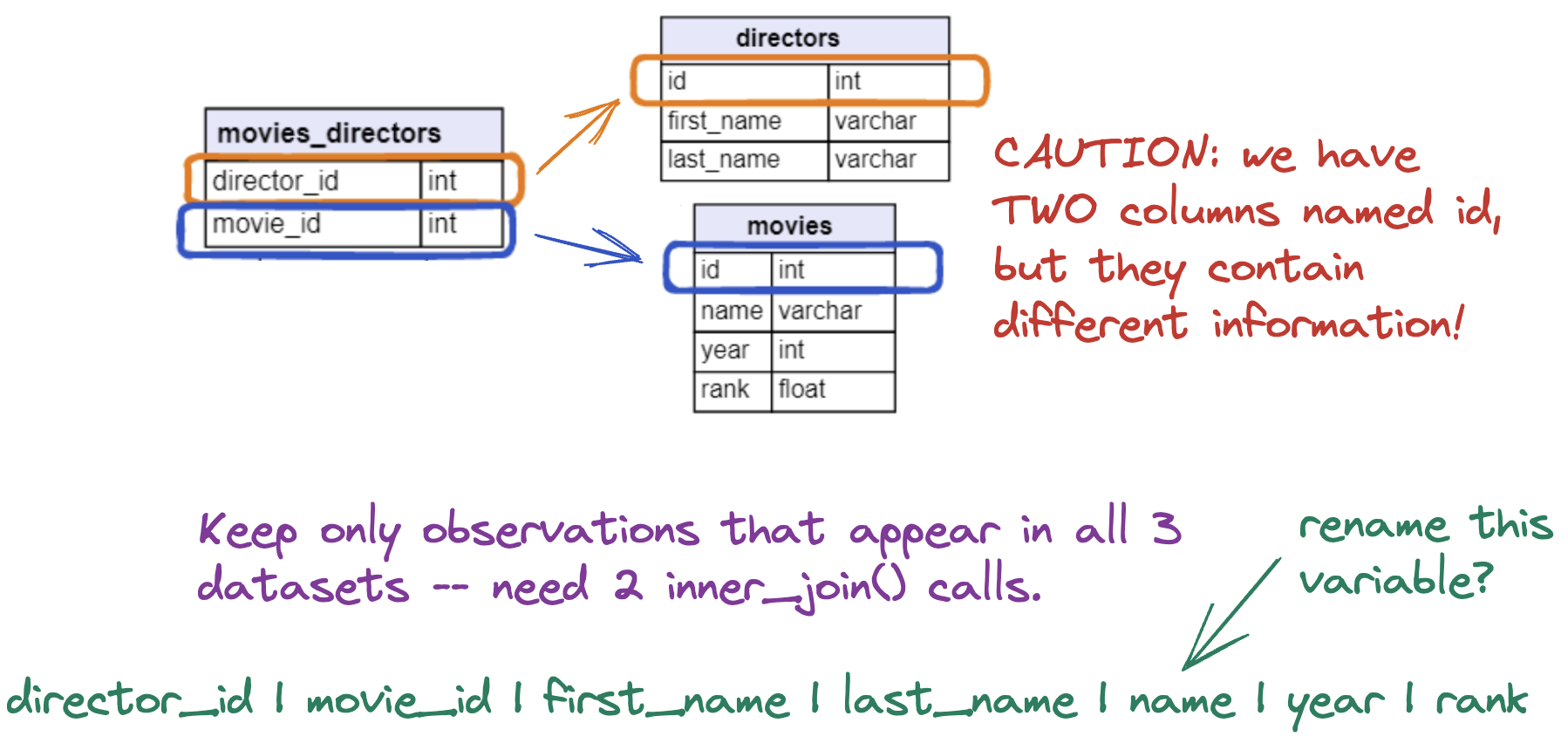
Discussion

Which datasets do we need to use to answer this question?

movies_directors |> 
  slice_head(n = 4)

director_id	movie_id
429	300229
2931	254943
9247	124110
11652	10920

directors |> 
  slice_head(n = 4)

id	first_name	last_name
429	Andrew	Adamson
2931	Darren	Aronofsky
9247	Zach	Braff
11652	James (I)	Cameron

movies |> 
  slice_head(n = 4)

id	name	year	rank
10920	Aliens	1986	8.2
17173	Animal House	1978	7.5
18979	Apollo 13	1995	7.5
30959	Batman Begins	2005	NA

movies_directors |> 
  inner_join(directors, 
             join_by(director_id == id))

director_id	movie_id	first_name	last_name
429	300229	Andrew	Adamson
2931	254943	Darren	Aronofsky
9247	124110	Zach	Braff
11652	10920	James (I)	Cameron
11652	333856	James (I)	Cameron
14927	192017	Ron	Clements
15092	109093	Ethan	Coen
15092	237431	Ethan	Coen
15093	109093	Joel	Coen
15093	237431	Joel	Coen
15901	130128	Francis Ford	Coppola
15906	194874	Sofia	Coppola
16816	350424	Cameron	Crowe
17810	297838	Frank	Darabont
22104	224842	Clint	Eastwood
24758	112290	David	Fincher
28395	46169	Mel (I)	Gibson
35573	18979	Ron	Howard
35838	257264	John (I)	Hughes
37872	300229	Vicky	Jenson
38746	238695	Mike (I)	Judge
41975	314965	David	Koepp
44291	17173	John (I)	Landis
46315	344203	Jay	Levey
48115	313459	George	Lucas
56332	192017	John	Musker
58201	30959	Christopher	Nolan
58201	210511	Christopher	Nolan
65940	111813	Rob	Reiner
66849	306032	Guy	Ritchie
68161	116907	Herbert (I)	Ross
74758	238072	Steven	Soderbergh
76524	167324	Oliver (I)	Stone
78273	176711	Quentin	Tarantino
78273	176712	Quentin	Tarantino
78273	267038	Quentin	Tarantino
78273	276217	Quentin	Tarantino
82525	147603	Paul (I)	Verhoeven
83616	207992	Andy	Wachowski
83617	207992	Larry	Wachowski
88802	256630	Unknown	Director

movies_directors |> 
  inner_join(directors, 
             join_by(director_id == id)) |> 
  inner_join(movies,
             join_by(movie_id == id))

director_id	movie_id	first_name	last_name	name	year	rank
429	300229	Andrew	Adamson	Shrek	2001	8.1
2931	254943	Darren	Aronofsky	Pi	1998	7.5
9247	124110	Zach	Braff	Garden State	2004	8.3
11652	10920	James (I)	Cameron	Aliens	1986	8.2
11652	333856	James (I)	Cameron	Titanic	1997	6.9
14927	192017	Ron	Clements	Little Mermaid, The	1989	7.3
15092	109093	Ethan	Coen	Fargo	1996	8.2
15092	237431	Ethan	Coen	O Brother, Where Art Thou?	2000	7.8
15093	109093	Joel	Coen	Fargo	1996	8.2
15093	237431	Joel	Coen	O Brother, Where Art Thou?	2000	7.8
15901	130128	Francis Ford	Coppola	Godfather, The	1972	9.0
15906	194874	Sofia	Coppola	Lost in Translation	2003	8.0
16816	350424	Cameron	Crowe	Vanilla Sky	2001	6.9
17810	297838	Frank	Darabont	Shawshank Redemption, The	1994	9.0
22104	224842	Clint	Eastwood	Mystic River	2003	8.1
24758	112290	David	Fincher	Fight Club	1999	8.5
28395	46169	Mel (I)	Gibson	Braveheart	1995	8.3
35573	18979	Ron	Howard	Apollo 13	1995	7.5
35838	257264	John (I)	Hughes	Planes, Trains & Automobiles	1987	7.2
37872	300229	Vicky	Jenson	Shrek	2001	8.1
38746	238695	Mike (I)	Judge	Office Space	1999	7.6
41975	314965	David	Koepp	Stir of Echoes	1999	7.0
44291	17173	John (I)	Landis	Animal House	1978	7.5
46315	344203	Jay	Levey	UHF	1989	6.6
48115	313459	George	Lucas	Star Wars	1977	8.8
56332	192017	John	Musker	Little Mermaid, The	1989	7.3
58201	30959	Christopher	Nolan	Batman Begins	2005	NA
58201	210511	Christopher	Nolan	Memento	2000	8.7
65940	111813	Rob	Reiner	Few Good Men, A	1992	7.5
66849	306032	Guy	Ritchie	Snatch.	2000	7.9
68161	116907	Herbert (I)	Ross	Footloose	1984	5.8
74758	238072	Steven	Soderbergh	Ocean's Eleven	2001	7.5
76524	167324	Oliver (I)	Stone	JFK	1991	7.8
78273	176711	Quentin	Tarantino	Kill Bill: Vol. 1	2003	8.4
78273	176712	Quentin	Tarantino	Kill Bill: Vol. 2	2004	8.2
78273	267038	Quentin	Tarantino	Pulp Fiction	1994	8.7
78273	276217	Quentin	Tarantino	Reservoir Dogs	1992	8.3
82525	147603	Paul (I)	Verhoeven	Hollow Man	2000	5.3
83616	207992	Andy	Wachowski	Matrix, The	1999	8.5
83617	207992	Larry	Wachowski	Matrix, The	1999	8.5
88802	256630	Unknown	Director	Pirates of the Caribbean	2003	NA

movies_directors |> 
  inner_join(directors, 
             join_by(director_id == id)) |> 
  inner_join(movies,
             join_by(movie_id == id)) |> 
  group_by(first_name, last_name) |>
  summarize(start_year = min(year),
            end_year = max(year)) |> 
  mutate(n_years_active = end_year - start_year) |> 
  arrange(desc(n_years_active))

first_name	last_name	start_year	end_year	n_years_active
Quentin	Tarantino	1992	2004	12
James (I)	Cameron	1986	1997	11
Christopher	Nolan	2000	2005	5
Ethan	Coen	1996	2000	4
Joel	Coen	1996	2000	4
Andrew	Adamson	2001	2001	0
Andy	Wachowski	1999	1999	0
Cameron	Crowe	2001	2001	0
Clint	Eastwood	2003	2003	0
Darren	Aronofsky	1998	1998	0
David	Fincher	1999	1999	0
David	Koepp	1999	1999	0
Francis Ford	Coppola	1972	1972	0
Frank	Darabont	1994	1994	0
George	Lucas	1977	1977	0
Guy	Ritchie	2000	2000	0
Herbert (I)	Ross	1984	1984	0
Jay	Levey	1989	1989	0
John	Musker	1989	1989	0
John (I)	Hughes	1987	1987	0
John (I)	Landis	1978	1978	0
Larry	Wachowski	1999	1999	0
Mel (I)	Gibson	1995	1995	0
Mike (I)	Judge	1999	1999	0
Oliver (I)	Stone	1991	1991	0
Paul (I)	Verhoeven	2000	2000	0
Rob	Reiner	1992	1992	0
Ron	Clements	1989	1989	0
Ron	Howard	1995	1995	0
Sofia	Coppola	2003	2003	0
Steven	Soderbergh	2001	2001	0
Unknown	Director	2003	2003	0
Vicky	Jenson	2001	2001	0
Zach	Braff	2004	2004	0

Know Your Unique Observations!

Discussion

What is the observational unit after joining the directors and movies_directors by the director_id key? What happens for directors that have multiple movies in the movies_directors data?

directors |> 
  inner_join(movies_directors, 
             join_by(id == director_id))

id	first_name	last_name	movie_id
429	Andrew	Adamson	300229
2931	Darren	Aronofsky	254943
9247	Zach	Braff	124110
11652	James (I)	Cameron	10920
11652	James (I)	Cameron	333856
14927	Ron	Clements	192017
15092	Ethan	Coen	109093
15092	Ethan	Coen	237431
15093	Joel	Coen	109093
15093	Joel	Coen	237431
15901	Francis Ford	Coppola	130128
15906	Sofia	Coppola	194874
16816	Cameron	Crowe	350424
17810	Frank	Darabont	297838
22104	Clint	Eastwood	224842
24758	David	Fincher	112290
28395	Mel (I)	Gibson	46169
35573	Ron	Howard	18979
35838	John (I)	Hughes	257264
37872	Vicky	Jenson	300229
38746	Mike (I)	Judge	238695
41975	David	Koepp	314965
44291	John (I)	Landis	17173
46315	Jay	Levey	344203
48115	George	Lucas	313459
56332	John	Musker	192017
58201	Christopher	Nolan	30959
58201	Christopher	Nolan	210511
65940	Rob	Reiner	111813
66849	Guy	Ritchie	306032
68161	Herbert (I)	Ross	116907
74758	Steven	Soderbergh	238072
76524	Oliver (I)	Stone	167324
78273	Quentin	Tarantino	176711
78273	Quentin	Tarantino	176712
78273	Quentin	Tarantino	267038
78273	Quentin	Tarantino	276217
82525	Paul (I)	Verhoeven	147603
83616	Andy	Wachowski	207992
83617	Larry	Wachowski	207992
88802	Unknown	Director	256630

Know Your Unique Observations!

Remember the rodent data from Lab 2. Say we had separate datsets for measurements and species information:

Species
Measurements

species

genus	species	taxa	species_id
Dipodomys	merriami	Rodent	DM
Dipodomys	ordii	Rodent	DO
Perognathus	flavus	Rodent	PF
Chaetodipus	penicillatus	Rodent	PP
Peromyscus	eremicus	Rodent	PE
Onychomys	leucogaster	Rodent	OL
Reithrodontomys	megalotis	Rodent	RM
Dipodomys	spectabilis	Rodent	DS
Onychomys	torridus	Rodent	OT
Neotoma	albigula	Rodent	NL
Peromyscus	maniculatus	Rodent	PM
Sigmodon	hispidus	Rodent	SH
Reithrodontomys	fulvescens	Rodent	RF
Chaetodipus	baileyi	Rodent	PB

measurements

genus_name	species	sex	hindfoot_length	weight
Dipodomys	merriami	M	35	40
Dipodomys	merriami	M	37	48
Dipodomys	merriami	F	34	29
Dipodomys	merriami	F	35	46
Dipodomys	merriami	M	35	36
Dipodomys	ordii	F	32	52
Perognathus	flavus	M	15	8
Dipodomys	merriami	F	36	35
Perognathus	flavus	M	12	7
Dipodomys	merriami	F	32	22
Perognathus	flavus	M	16	9
Dipodomys	merriami	F	34	42
Perognathus	flavus	F	14	8
Dipodomys	merriami	F	35	41
Dipodomys	merriami	F	37	37
Dipodomys	merriami	F	35	43
Dipodomys	merriami	F	35	41
Dipodomys	merriami	F	33	40
Perognathus	flavus	F	11	9
Dipodomys	merriami	F	35	45
Chaetodipus	penicillatus	F	20	15
Dipodomys	merriami	M	35	29
Dipodomys	merriami	M	35	39
Dipodomys	merriami	F	36	43
Dipodomys	merriami	M	38	46
Dipodomys	merriami	M	36	41
Dipodomys	merriami	M	36	41
Dipodomys	merriami	M	38	40
Dipodomys	merriami	M	37	45
Dipodomys	merriami	F	35	46
Dipodomys	merriami	F	35	40
Dipodomys	merriami	F	35	30
Dipodomys	merriami	M	35	39
Dipodomys	merriami	M	35	34
Dipodomys	merriami	F	37	42
Dipodomys	merriami	M	37	42
Perognathus	flavus	F	13	8
Dipodomys	merriami	F	37	31
Dipodomys	merriami	F	36	40
Dipodomys	merriami	M	36	37
Dipodomys	merriami	M	36	48
Dipodomys	merriami	M	37	42
Dipodomys	merriami	F	39	45
Chaetodipus	penicillatus	F	21	16
Dipodomys	merriami	F	36	36
Dipodomys	merriami	M	36	42
Dipodomys	merriami	M	36	44
Dipodomys	merriami	F	36	41
Dipodomys	merriami	F	36	40
Dipodomys	merriami	M	37	34
Dipodomys	merriami	M	33	40
Dipodomys	merriami	M	33	44
Dipodomys	merriami	M	37	44
Dipodomys	merriami	M	34	36
Dipodomys	merriami	M	35	33
Dipodomys	merriami	F	37	46
Dipodomys	merriami	F	34	35
Dipodomys	merriami	M	36	46
Dipodomys	merriami	F	33	37
Dipodomys	merriami	M	36	34
Dipodomys	merriami	F	36	45
Perognathus	flavus	F	15	7
Dipodomys	merriami	M	37	51
Dipodomys	merriami	M	35	39
Dipodomys	merriami	M	36	29
Dipodomys	merriami	F	32	48
Dipodomys	merriami	M	38	46
Dipodomys	merriami	F	37	41
Dipodomys	merriami	M	37	45
Dipodomys	merriami	F	35	42
Dipodomys	merriami	F	36	53
Dipodomys	merriami	F	35	49
Dipodomys	merriami	F	36	46
Perognathus	flavus	F	13	9
Chaetodipus	penicillatus	F	19	15
Perognathus	flavus	M	13	4
Dipodomys	merriami	M	36	48
Dipodomys	merriami	M	37	51
Dipodomys	merriami	M	38	50
Dipodomys	merriami	M	35	44
Dipodomys	merriami	M	25	44
Dipodomys	merriami	M	35	45
Dipodomys	merriami	F	37	45
Peromyscus	eremicus	M	20	19
Dipodomys	merriami	F	38	44
Dipodomys	merriami	F	36	42
Dipodomys	merriami	M	37	39
Dipodomys	merriami	M	37	47
Dipodomys	merriami	M	36	42
Dipodomys	merriami	M	36	49
Dipodomys	merriami	M	38	39
Dipodomys	merriami	F	36	43
Dipodomys	merriami	M	35	50
Dipodomys	merriami	M	36	41
Dipodomys	merriami	M	37	47
Dipodomys	merriami	F	36	37
Dipodomys	merriami	M	36	41
Dipodomys	merriami	F	36	36
Dipodomys	merriami	M	36	45
Peromyscus	eremicus	M	19	20

Know Your Unique Observations!

Discussion

What happens if we join species and measurements by the genus only?

measurements |> 
  inner_join(species, 
             by = join_by(genus_name == genus))

genus_name	species.x	sex	hindfoot_length	weight	species.y	taxa	species_id
Dipodomys	merriami	M	35	40	merriami	Rodent	DM
Dipodomys	merriami	M	35	40	ordii	Rodent	DO
Dipodomys	merriami	M	35	40	spectabilis	Rodent	DS
Dipodomys	merriami	M	37	48	merriami	Rodent	DM
Dipodomys	merriami	M	37	48	ordii	Rodent	DO
Dipodomys	merriami	M	37	48	spectabilis	Rodent	DS
Dipodomys	merriami	F	34	29	merriami	Rodent	DM
Dipodomys	merriami	F	34	29	ordii	Rodent	DO
Dipodomys	merriami	F	34	29	spectabilis	Rodent	DS
Dipodomys	merriami	F	35	46	merriami	Rodent	DM
Dipodomys	merriami	F	35	46	ordii	Rodent	DO
Dipodomys	merriami	F	35	46	spectabilis	Rodent	DS
Dipodomys	merriami	M	35	36	merriami	Rodent	DM
Dipodomys	merriami	M	35	36	ordii	Rodent	DO
Dipodomys	merriami	M	35	36	spectabilis	Rodent	DS
Dipodomys	ordii	F	32	52	merriami	Rodent	DM
Dipodomys	ordii	F	32	52	ordii	Rodent	DO
Dipodomys	ordii	F	32	52	spectabilis	Rodent	DS
Perognathus	flavus	M	15	8	flavus	Rodent	PF
Dipodomys	merriami	F	36	35	merriami	Rodent	DM
Dipodomys	merriami	F	36	35	ordii	Rodent	DO
Dipodomys	merriami	F	36	35	spectabilis	Rodent	DS
Perognathus	flavus	M	12	7	flavus	Rodent	PF
Dipodomys	merriami	F	32	22	merriami	Rodent	DM
Dipodomys	merriami	F	32	22	ordii	Rodent	DO
Dipodomys	merriami	F	32	22	spectabilis	Rodent	DS
Perognathus	flavus	M	16	9	flavus	Rodent	PF
Dipodomys	merriami	F	34	42	merriami	Rodent	DM
Dipodomys	merriami	F	34	42	ordii	Rodent	DO
Dipodomys	merriami	F	34	42	spectabilis	Rodent	DS
Perognathus	flavus	F	14	8	flavus	Rodent	PF
Dipodomys	merriami	F	35	41	merriami	Rodent	DM
Dipodomys	merriami	F	35	41	ordii	Rodent	DO
Dipodomys	merriami	F	35	41	spectabilis	Rodent	DS
Dipodomys	merriami	F	37	37	merriami	Rodent	DM
Dipodomys	merriami	F	37	37	ordii	Rodent	DO
Dipodomys	merriami	F	37	37	spectabilis	Rodent	DS
Dipodomys	merriami	F	35	43	merriami	Rodent	DM
Dipodomys	merriami	F	35	43	ordii	Rodent	DO
Dipodomys	merriami	F	35	43	spectabilis	Rodent	DS
Dipodomys	merriami	F	35	41	merriami	Rodent	DM
Dipodomys	merriami	F	35	41	ordii	Rodent	DO
Dipodomys	merriami	F	35	41	spectabilis	Rodent	DS
Dipodomys	merriami	F	33	40	merriami	Rodent	DM
Dipodomys	merriami	F	33	40	ordii	Rodent	DO
Dipodomys	merriami	F	33	40	spectabilis	Rodent	DS
Perognathus	flavus	F	11	9	flavus	Rodent	PF
Dipodomys	merriami	F	35	45	merriami	Rodent	DM
Dipodomys	merriami	F	35	45	ordii	Rodent	DO
Dipodomys	merriami	F	35	45	spectabilis	Rodent	DS
Chaetodipus	penicillatus	F	20	15	penicillatus	Rodent	PP
Chaetodipus	penicillatus	F	20	15	baileyi	Rodent	PB
Dipodomys	merriami	M	35	29	merriami	Rodent	DM
Dipodomys	merriami	M	35	29	ordii	Rodent	DO
Dipodomys	merriami	M	35	29	spectabilis	Rodent	DS
Dipodomys	merriami	M	35	39	merriami	Rodent	DM
Dipodomys	merriami	M	35	39	ordii	Rodent	DO
Dipodomys	merriami	M	35	39	spectabilis	Rodent	DS
Dipodomys	merriami	F	36	43	merriami	Rodent	DM
Dipodomys	merriami	F	36	43	ordii	Rodent	DO
Dipodomys	merriami	F	36	43	spectabilis	Rodent	DS
Dipodomys	merriami	M	38	46	merriami	Rodent	DM
Dipodomys	merriami	M	38	46	ordii	Rodent	DO
Dipodomys	merriami	M	38	46	spectabilis	Rodent	DS
Dipodomys	merriami	M	36	41	merriami	Rodent	DM
Dipodomys	merriami	M	36	41	ordii	Rodent	DO
Dipodomys	merriami	M	36	41	spectabilis	Rodent	DS
Dipodomys	merriami	M	36	41	merriami	Rodent	DM
Dipodomys	merriami	M	36	41	ordii	Rodent	DO
Dipodomys	merriami	M	36	41	spectabilis	Rodent	DS
Dipodomys	merriami	M	38	40	merriami	Rodent	DM
Dipodomys	merriami	M	38	40	ordii	Rodent	DO
Dipodomys	merriami	M	38	40	spectabilis	Rodent	DS
Dipodomys	merriami	M	37	45	merriami	Rodent	DM
Dipodomys	merriami	M	37	45	ordii	Rodent	DO
Dipodomys	merriami	M	37	45	spectabilis	Rodent	DS
Dipodomys	merriami	F	35	46	merriami	Rodent	DM
Dipodomys	merriami	F	35	46	ordii	Rodent	DO
Dipodomys	merriami	F	35	46	spectabilis	Rodent	DS
Dipodomys	merriami	F	35	40	merriami	Rodent	DM
Dipodomys	merriami	F	35	40	ordii	Rodent	DO
Dipodomys	merriami	F	35	40	spectabilis	Rodent	DS
Dipodomys	merriami	F	35	30	merriami	Rodent	DM
Dipodomys	merriami	F	35	30	ordii	Rodent	DO
Dipodomys	merriami	F	35	30	spectabilis	Rodent	DS
Dipodomys	merriami	M	35	39	merriami	Rodent	DM
Dipodomys	merriami	M	35	39	ordii	Rodent	DO
Dipodomys	merriami	M	35	39	spectabilis	Rodent	DS
Dipodomys	merriami	M	35	34	merriami	Rodent	DM
Dipodomys	merriami	M	35	34	ordii	Rodent	DO
Dipodomys	merriami	M	35	34	spectabilis	Rodent	DS
Dipodomys	merriami	F	37	42	merriami	Rodent	DM
Dipodomys	merriami	F	37	42	ordii	Rodent	DO
Dipodomys	merriami	F	37	42	spectabilis	Rodent	DS
Dipodomys	merriami	M	37	42	merriami	Rodent	DM
Dipodomys	merriami	M	37	42	ordii	Rodent	DO
Dipodomys	merriami	M	37	42	spectabilis	Rodent	DS
Perognathus	flavus	F	13	8	flavus	Rodent	PF
Dipodomys	merriami	F	37	31	merriami	Rodent	DM
Dipodomys	merriami	F	37	31	ordii	Rodent	DO

DANGER : MANY-TO-MANY JOIN!

Our observations exploded and the species_id isn’t even right for some observations! We also now have a species.x and species.y variable since the variable was present in both the left and right data.

Joining on Multiple Variables

To fix this, we need to join on multiple variables (a compound key):

species |> 
  full_join(measurements,
            join_by(species == species, 
                    genus == genus_name))

genus	species	taxa	species_id	sex	hindfoot_length	weight
Dipodomys	merriami	Rodent	DM	M	35	40
Dipodomys	merriami	Rodent	DM	M	37	48
Dipodomys	merriami	Rodent	DM	F	34	29
Dipodomys	merriami	Rodent	DM	F	35	46
Dipodomys	merriami	Rodent	DM	M	35	36
Dipodomys	merriami	Rodent	DM	F	36	35
Dipodomys	merriami	Rodent	DM	F	32	22
Dipodomys	merriami	Rodent	DM	F	34	42
Dipodomys	merriami	Rodent	DM	F	35	41
Dipodomys	merriami	Rodent	DM	F	37	37
Dipodomys	merriami	Rodent	DM	F	35	43
Dipodomys	merriami	Rodent	DM	F	35	41
Dipodomys	merriami	Rodent	DM	F	33	40
Dipodomys	merriami	Rodent	DM	F	35	45
Dipodomys	merriami	Rodent	DM	M	35	29
Dipodomys	merriami	Rodent	DM	M	35	39
Dipodomys	merriami	Rodent	DM	F	36	43
Dipodomys	merriami	Rodent	DM	M	38	46
Dipodomys	merriami	Rodent	DM	M	36	41
Dipodomys	merriami	Rodent	DM	M	36	41
Dipodomys	merriami	Rodent	DM	M	38	40
Dipodomys	merriami	Rodent	DM	M	37	45
Dipodomys	merriami	Rodent	DM	F	35	46
Dipodomys	merriami	Rodent	DM	F	35	40
Dipodomys	merriami	Rodent	DM	F	35	30
Dipodomys	merriami	Rodent	DM	M	35	39
Dipodomys	merriami	Rodent	DM	M	35	34
Dipodomys	merriami	Rodent	DM	F	37	42
Dipodomys	merriami	Rodent	DM	M	37	42
Dipodomys	merriami	Rodent	DM	F	37	31
Dipodomys	merriami	Rodent	DM	F	36	40
Dipodomys	merriami	Rodent	DM	M	36	37
Dipodomys	merriami	Rodent	DM	M	36	48
Dipodomys	merriami	Rodent	DM	M	37	42
Dipodomys	merriami	Rodent	DM	F	39	45
Dipodomys	merriami	Rodent	DM	F	36	36
Dipodomys	merriami	Rodent	DM	M	36	42
Dipodomys	merriami	Rodent	DM	M	36	44
Dipodomys	merriami	Rodent	DM	F	36	41
Dipodomys	merriami	Rodent	DM	F	36	40
Dipodomys	merriami	Rodent	DM	M	37	34
Dipodomys	merriami	Rodent	DM	M	33	40
Dipodomys	merriami	Rodent	DM	M	33	44
Dipodomys	merriami	Rodent	DM	M	37	44
Dipodomys	merriami	Rodent	DM	M	34	36
Dipodomys	merriami	Rodent	DM	M	35	33
Dipodomys	merriami	Rodent	DM	F	37	46
Dipodomys	merriami	Rodent	DM	F	34	35
Dipodomys	merriami	Rodent	DM	M	36	46
Dipodomys	merriami	Rodent	DM	F	33	37
Dipodomys	merriami	Rodent	DM	M	36	34
Dipodomys	merriami	Rodent	DM	F	36	45
Dipodomys	merriami	Rodent	DM	M	37	51
Dipodomys	merriami	Rodent	DM	M	35	39
Dipodomys	merriami	Rodent	DM	M	36	29
Dipodomys	merriami	Rodent	DM	F	32	48
Dipodomys	merriami	Rodent	DM	M	38	46
Dipodomys	merriami	Rodent	DM	F	37	41
Dipodomys	merriami	Rodent	DM	M	37	45
Dipodomys	merriami	Rodent	DM	F	35	42
Dipodomys	merriami	Rodent	DM	F	36	53
Dipodomys	merriami	Rodent	DM	F	35	49
Dipodomys	merriami	Rodent	DM	F	36	46
Dipodomys	merriami	Rodent	DM	M	36	48
Dipodomys	merriami	Rodent	DM	M	37	51
Dipodomys	merriami	Rodent	DM	M	38	50
Dipodomys	merriami	Rodent	DM	M	35	44
Dipodomys	merriami	Rodent	DM	M	25	44
Dipodomys	merriami	Rodent	DM	M	35	45
Dipodomys	merriami	Rodent	DM	F	37	45
Dipodomys	merriami	Rodent	DM	F	38	44
Dipodomys	merriami	Rodent	DM	F	36	42
Dipodomys	merriami	Rodent	DM	M	37	39
Dipodomys	merriami	Rodent	DM	M	37	47
Dipodomys	merriami	Rodent	DM	M	36	42
Dipodomys	merriami	Rodent	DM	M	36	49
Dipodomys	merriami	Rodent	DM	M	38	39
Dipodomys	merriami	Rodent	DM	F	36	43
Dipodomys	merriami	Rodent	DM	M	35	50
Dipodomys	merriami	Rodent	DM	M	36	41
Dipodomys	merriami	Rodent	DM	M	37	47
Dipodomys	merriami	Rodent	DM	F	36	37
Dipodomys	merriami	Rodent	DM	M	36	41
Dipodomys	merriami	Rodent	DM	F	36	36
Dipodomys	merriami	Rodent	DM	M	36	45
Dipodomys	merriami	Rodent	DM	M	37	40
Dipodomys	merriami	Rodent	DM	M	38	49
Dipodomys	merriami	Rodent	DM	F	36	55
Dipodomys	merriami	Rodent	DM	M	37	46
Dipodomys	merriami	Rodent	DM	F	36	38
Dipodomys	merriami	Rodent	DM	M	37	44
Dipodomys	merriami	Rodent	DM	M	37	41
Dipodomys	merriami	Rodent	DM	M	37	46
Dipodomys	merriami	Rodent	DM	M	34	36
Dipodomys	merriami	Rodent	DM	M	37	44
Dipodomys	merriami	Rodent	DM	M	36	53
Dipodomys	merriami	Rodent	DM	M	38	41
Dipodomys	merriami	Rodent	DM	M	37	48
Dipodomys	merriami	Rodent	DM	M	38	47
Dipodomys	merriami	Rodent	DM	F	36	42

Factor Variables

What is a factor variable?

Factors are used for

categorical variables with a fixed and known set of possible values.

E.g., day_born = Sunday, Monday, Tuesday, …, Saturday

displaying character vectors in non-alphabetical order.

useful for nice tables and plots!

Eras Tour

Let’s consider songs that Taylor Swift played on her Eras Tour.

I have randomly selected 25 songs (and their albums) to demonstrate.

eras_data |> 
  slice_head(n = 10)

Song	Album
22	Red
...Ready for It?	Reputation
The Archer	Lover
Bejeweled	Midnights
Style	1989
You Belong With Me	Fearless
Don't Blame Me	Reputation
illicit affairs	Folklore
Lavender Haze	Midnights
marjorie	Evermore

Creating a Factor – Base `R`

A character vector:

eras_data |> 
  pull(Album)

 [1] "Red"        "Reputation" "Lover"      "Midnights"  "1989"      
 [6] "Fearless"   "Reputation" "Folklore"   "Midnights"  "Evermore"  
[11] "Evermore"   "Lover"      "Lover"      "Red"        "Reputation"
[16] "Reputation" "Speak Now"  "Red"        "Midnights"  "Fearless"  
[21] "1989"       "Midnights"  "Fearless"   "Folklore"   "Lover"

A factor vector:

eras_data |> 
  pull(Album) |> 
  factor()

 [1] Red        Reputation Lover      Midnights  1989       Fearless  
 [7] Reputation Folklore   Midnights  Evermore   Evermore   Lover     
[13] Lover      Red        Reputation Reputation Speak Now  Red       
[19] Midnights  Fearless   1989       Midnights  Fearless   Folklore  
[25] Lover     
9 Levels: 1989 Evermore Fearless Folklore Lover Midnights Red ... Speak Now

Creating a Factor – Base `R`

When you create a factor variable from a vector…

Every unique element in the vector becomes a level.
The levels are ordered alphabetically.
The elements are no longer displayed in quotes.

Creating a Factor – Base `R`

You can specify the order of the levels with the level argument.

eras_data |> 
  pull(Album) |> 
  factor(levels = c("Fearless","Speak Now","Red","1989",
                    "Reputation","Lover","Folklore",
                    "Evermore","Midnights"))

 [1] Red        Reputation Lover      Midnights  1989       Fearless  
 [7] Reputation Folklore   Midnights  Evermore   Evermore   Lover     
[13] Lover      Red        Reputation Reputation Speak Now  Red       
[19] Midnights  Fearless   1989       Midnights  Fearless   Folklore  
[25] Lover     
9 Levels: Fearless Speak Now Red 1989 Reputation Lover Folklore ... Midnights

`forcats`

We use this package to…

turn character variables into factors.
make factors by discretizing numeric variables.
rename or reorder the levels of an existing factor.

Note

The packages forcats (“for categoricals”) helps wrangle categorical variables.

forcats loads with tidyverse!

Creating a Factor – `fct`

With fct(), the levels are automatically ordered in the order of first appearance.

eras_data |> 
  mutate(Album = fct(Album)) |> 
  pull(Album)

 [1] Red        Reputation Lover      Midnights  1989       Fearless  
 [7] Reputation Folklore   Midnights  Evermore   Evermore   Lover     
[13] Lover      Red        Reputation Reputation Speak Now  Red       
[19] Midnights  Fearless   1989       Midnights  Fearless   Folklore  
[25] Lover     
9 Levels: Red Reputation Lover Midnights 1989 Fearless Folklore ... Speak Now

Creating a Factor – `fct`

You can still specify the order of the levels with level.

eras_data |> 
  mutate(Album = fct(Album,
                     levels = c("Fearless","Speak Now","Red",
                                "1989", "Reputation","Lover",
                                "Folklore", "Evermore","Midnights"))) |> 
  pull(Album)

 [1] Red        Reputation Lover      Midnights  1989       Fearless  
 [7] Reputation Folklore   Midnights  Evermore   Evermore   Lover     
[13] Lover      Red        Reputation Reputation Speak Now  Red       
[19] Midnights  Fearless   1989       Midnights  Fearless   Folklore  
[25] Lover     
9 Levels: Fearless Speak Now Red 1989 Reputation Lover Folklore ... Midnights

Creating a Factor – `fct`

You can also specify non-present levels.

eras_data |> 
  mutate(Album = fct(Album, 
                     levels = c("Taylor Swift",
                                "Fearless","Speak Now","Red",
                                "1989", "Reputation","Lover",
                                "Folklore", "Evermore","Midnights",
                                "The Tortured Poets Department"))) |> 
  pull(Album)

 [1] Red        Reputation Lover      Midnights  1989       Fearless  
 [7] Reputation Folklore   Midnights  Evermore   Evermore   Lover     
[13] Lover      Red        Reputation Reputation Speak Now  Red       
[19] Midnights  Fearless   1989       Midnights  Fearless   Folklore  
[25] Lover     
11 Levels: Taylor Swift Fearless Speak Now Red 1989 Reputation ... The Tortured Poets Department

Re-coding a Factor – `fct_recode`

Oops, we have a typo in some of our levels! We change existing levels with the syntax <new level> = <old level>.

eras_data |>
  mutate(Album = fct_recode(.f = Album,
                            "folklore" = "Folklore",
                            "evermore" = "Evermore",
                            "reputation" = "Reputation")) |>
  pull(Album)

 [1] Red        reputation Lover      Midnights  1989       Fearless  
 [7] reputation folklore   Midnights  evermore   evermore   Lover     
[13] Lover      Red        reputation reputation Speak Now  Red       
[19] Midnights  Fearless   1989       Midnights  Fearless   folklore  
[25] Lover     
11 Levels: Taylor Swift Fearless Speak Now Red 1989 reputation ... The Tortured Poets Department

Non-specified levels are not re-coded.

Re-coding a Factor – `case_when`

We have similar functionality with the case_when() function…

eras_data |>
  mutate(Album = case_when(Album == "Folklore" ~ "folklore",
                           Album == "Evermore" ~ "evermore",
                           Album == "Reputation" ~ "reputation",
                           .default = Album),
         Album = fct(Album)) |> 
  pull(Album)

 [1] Red        reputation Lover      Midnights  1989       Fearless  
 [7] reputation folklore   Midnights  evermore   evermore   Lover     
[13] Lover      Red        reputation reputation Speak Now  Red       
[19] Midnights  Fearless   1989       Midnights  Fearless   folklore  
[25] Lover     
9 Levels: Red reputation Lover Midnights 1989 Fearless folklore ... Speak Now

Collapsing a Factor –`fct_collapse`

Collapse multiple existing levels of a factor with the syntax <new level> = c(<old levels>).

eras_data |> 
  mutate(Genre = fct_collapse(.f= Album,
                       "country pop" = c("Taylor Swift", "Fearless"),
                       "pop rock" = c("Speak Now","Red"),
                       "electropop" = c("1989","reputation","Lover"),
                       "folk pop" = c("folklore","evermore"),
                       "alt-pop" = "Midnights")) |> 
  slice_sample(n = 6)

Song	Album	Genre
willow	evermore	folk pop
You Belong With Me	Fearless	country pop
Lavender Haze	Midnights	alt-pop
We Are Never Ever Getting Back Together	Red	pop rock
illicit affairs	folklore	folk pop
Look What You Made Me Do	reputation	electropop

Re-leveling a Factor –`fct_relevel`

Change the order of the levels of an existing factor.

Original
Ordered by Copies Sold

eras_data |>
  pull(Album) |> 
  levels()

 [1] "Taylor Swift"                  "Fearless"                     
 [3] "Speak Now"                     "Red"                          
 [5] "1989"                          "reputation"                   
 [7] "Lover"                         "folklore"                     
 [9] "evermore"                      "Midnights"                    
[11] "The Tortured Poets Department"

eras_data |> 
  mutate(Album = fct_relevel(.f = Album, 
                             c("Fearless","1989","Taylor Swift",
                               "Speak Now","Red","Midnights","reputation",
                               "folklore","Lover","evermore"))) |>
  pull(Album) |>
  levels()

 [1] "Fearless"                      "1989"                         
 [3] "Taylor Swift"                  "Speak Now"                    
 [5] "Red"                           "Midnights"                    
 [7] "reputation"                    "folklore"                     
 [9] "Lover"                         "evermore"                     
[11] "The Tortured Poets Department"

Unspecified levels remain in the same order at the end.

Re-ordering Factors in `ggplot2`

Original
Plot
Specify Levels
Plot

The bars follow the default factor levels.

full_eras |> 
  mutate(Album = fct(Album)) |> 
  ggplot() +
  geom_bar(aes(y = Album), fill = "#A5C9A5") +
  theme_minimal() +
  labs(x = "Number of Songs",
       y = "",
       subtitle = "Album",
       title = "Songs Played on the Eras Tour")

We can order factor levels to order the bar plot.

full_eras |> 
  mutate(Album = fct(Album,
                     levels = c("Fearless","Speak Now","Red",
                                "1989","Reputation","Lover",
                                "Folklore","Evermore",
                                "Midnights"))) |> 
  ggplot() +
  geom_bar(aes(y = Album), fill = "#A5C9A5") +
  theme_minimal() +
  labs(x = "Number of Songs",
       y = "",
       subtitle = "Album",
       title = "Songs Played on the Eras Tour")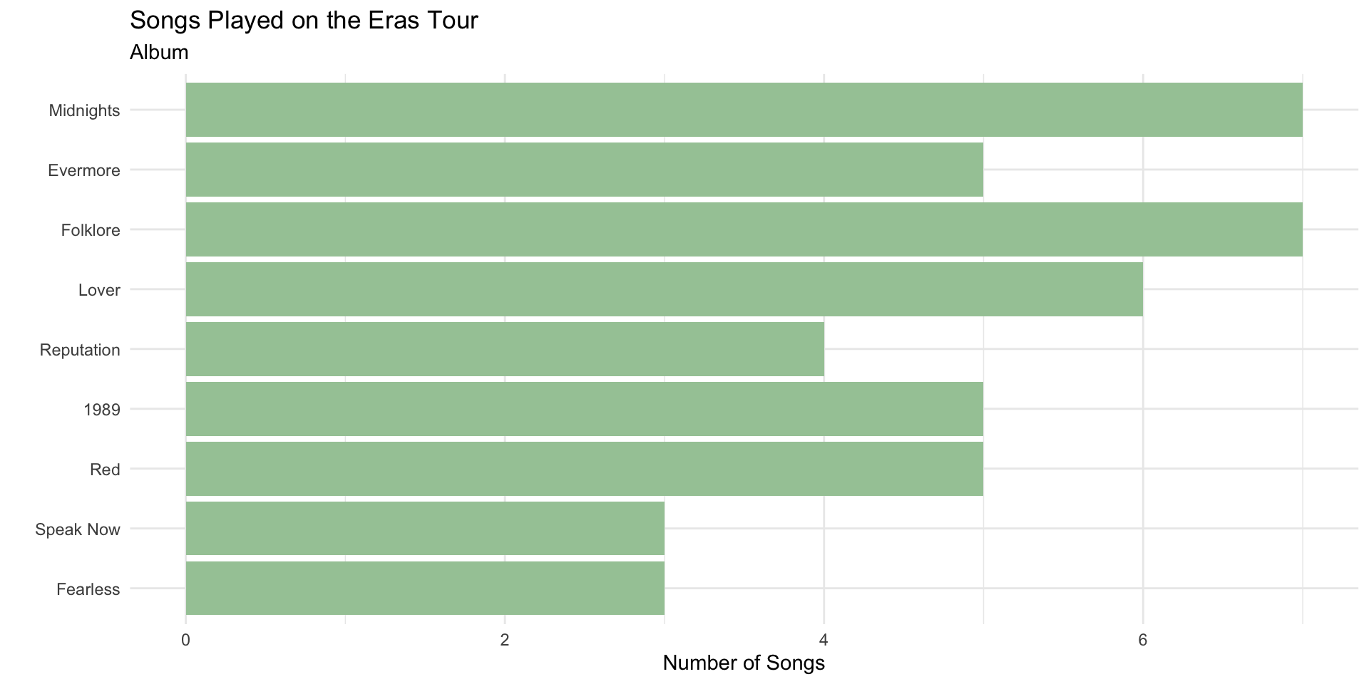

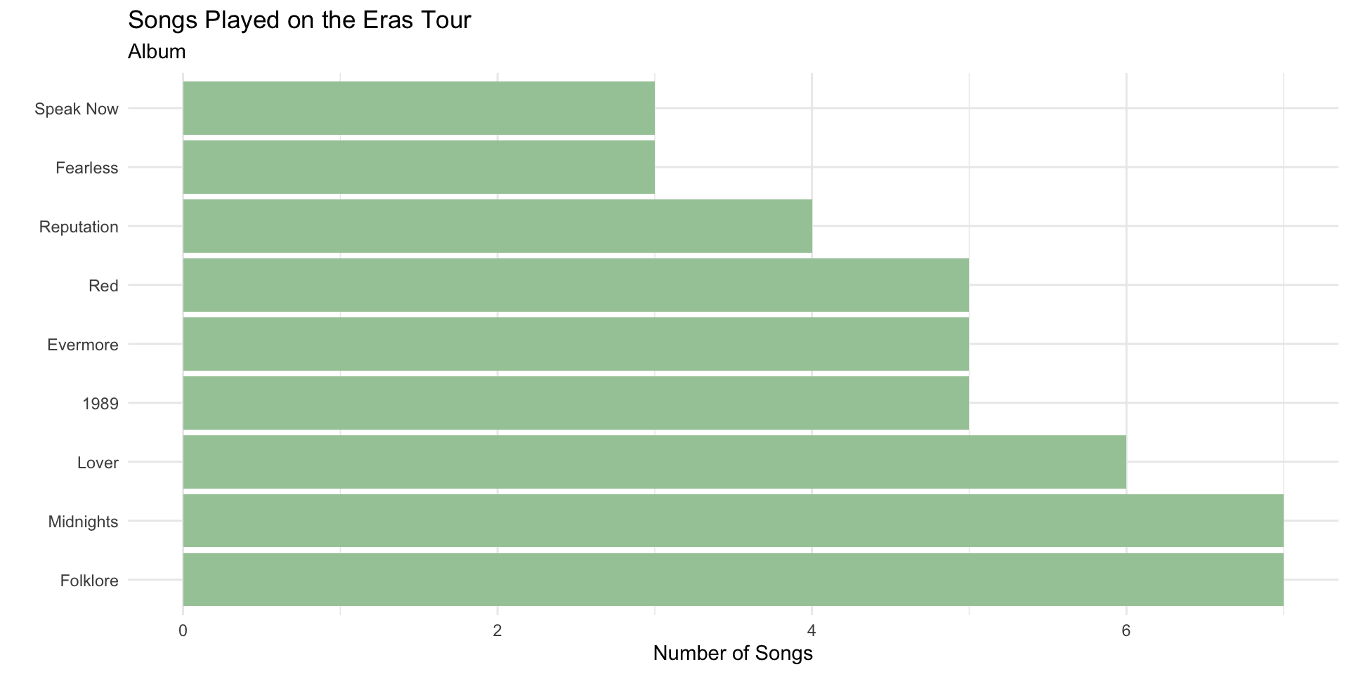
Re-ordering Factors in `ggplot2`

Original
Plot
Reorder by Value
Plot

The bars follow the default factor levels.

full_eras |> 
  mutate(Album = fct(Album)) |> 
  ggplot() +
  geom_bar(aes(y = Album), fill = "#A5C9A5") +
  theme_minimal() +
  labs(x = "Number of Songs",
       y = "",
       subtitle = "Album",
       title = "Songs Played on the Eras Tour")

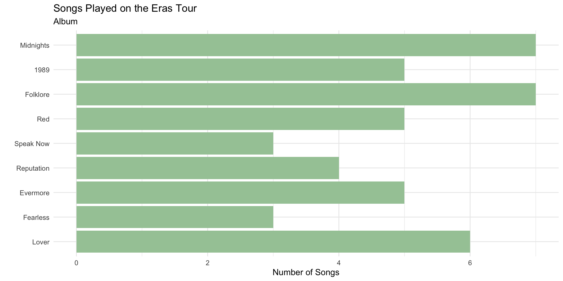
We can order factor levels to order the bar plot by the count using fct_infreq()

full_eras |> 
  ggplot() +
  geom_bar(aes(y = fct_infreq(Album)), 
           fill = "#A5C9A5") +
  theme_minimal() +
  labs(x = "Number of Songs",
       y = "",
       subtitle = "Album",
       title = "Songs Played on the Eras Tour")

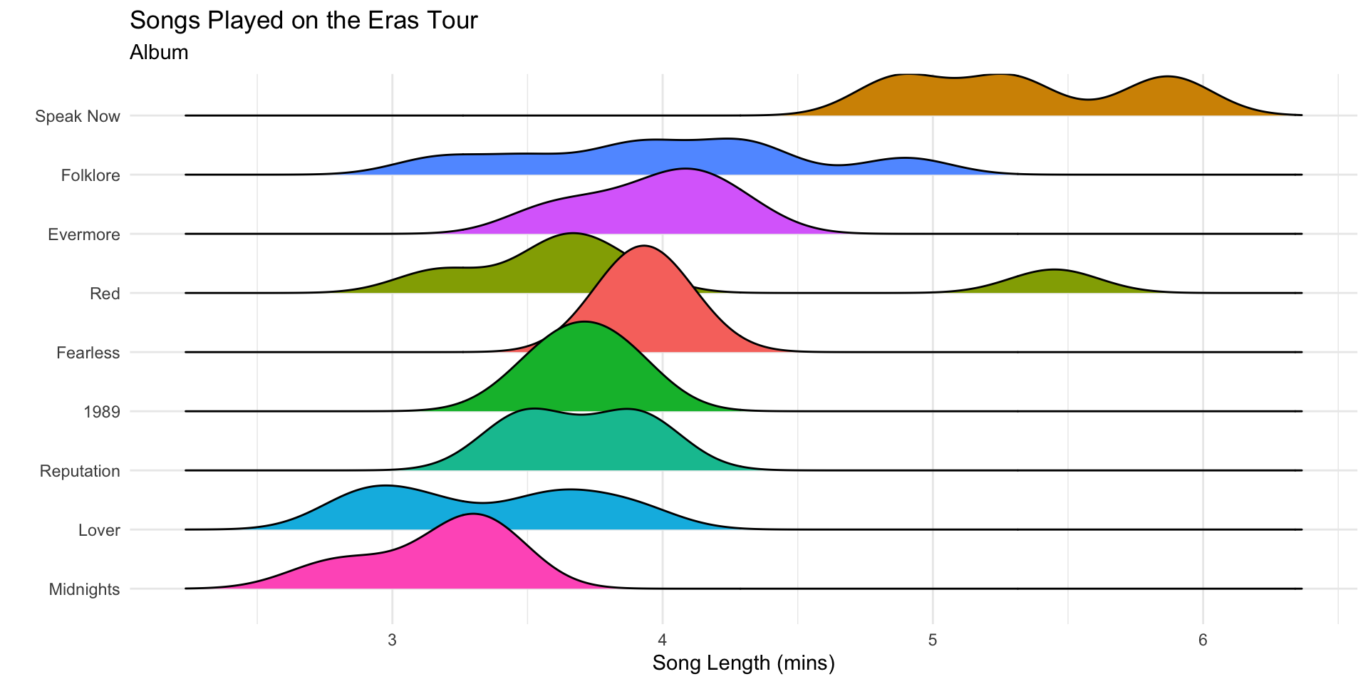
Re-ordering Factors in `ggplot2`

Original
Plot
fct_reorder()
Plot

The ridge plots follow the order of the factor levels.

full_eras |> 
  ggplot(aes(x = Length, 
             y = Album, 
             fill = Album)) +
  geom_density_ridges() +
  theme_minimal() +
  theme(legend.position = "none")+
  labs(x = "Song Length (mins)",
       y = "",
       subtitle = "Album",
       title = "Songs Played on the Eras Tour")

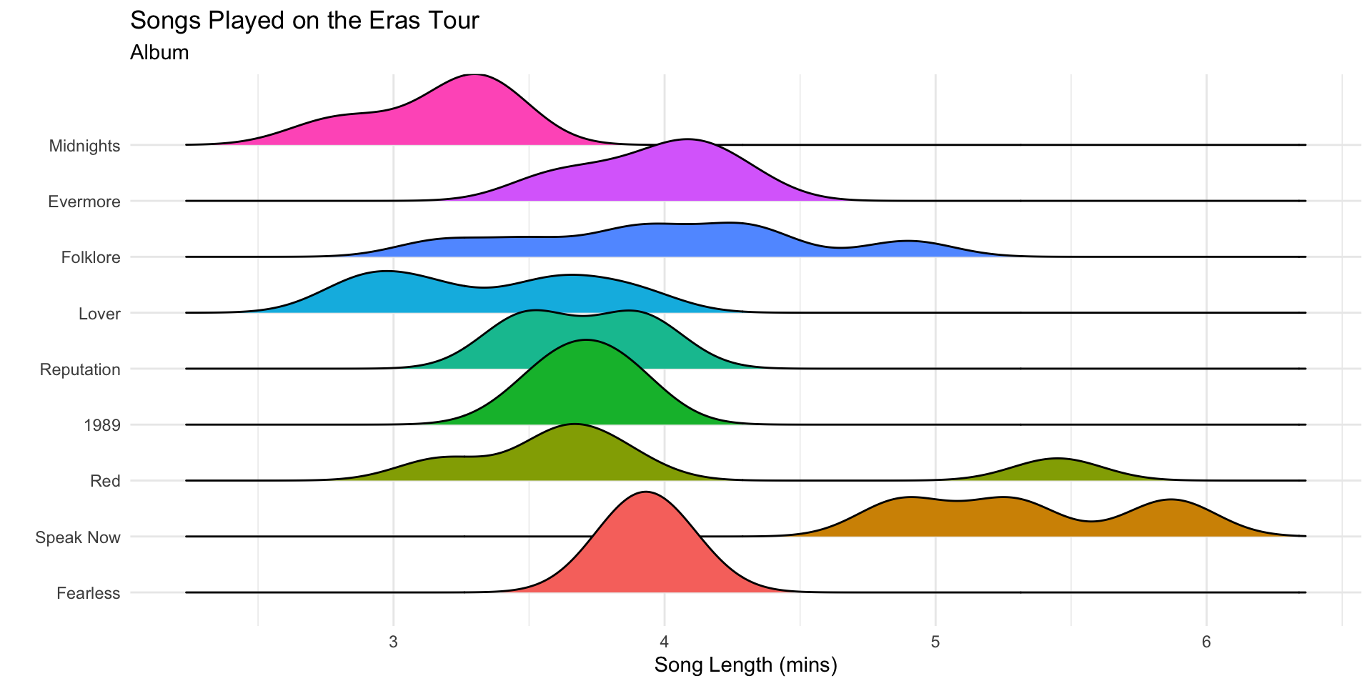
Inside ggplot(), we can order factor levels by a summary value.

full_eras |> 
  ggplot(aes(x = Length, 
             y = fct_reorder(.f = Album,
                             .x = Length,
                             .fun = mean), 
             fill = Album)) +
  geom_density_ridges() +
  theme_minimal() +
  theme(legend.position = "none")+
  labs(x = "Song Length (mins)",
       y = "",
       subtitle = "Album",
       title = "Songs Played on the Eras Tour")

Re-ordering Factors in `ggplot2`

Original
Plot
fct_reorder2()
Plot

Remember the miliary data from the practice activity?

The legend follows the order of the factor levels.

military_long |> 
  filter(Country %in% central.asia,
         !is.na(spending)) |> 
  ggplot(aes(x = year,
             y = spending,
             color = Country)) +
  geom_line() +
  labs(x = "Year",
       y = "",
       subtitle = "Spending (as % of Government Spending)",
       title = "Military Expenditures in Central Asia") +
  scale_color_manual(values = brewer.pal(3, "Dark2")) +
  scale_y_continuous(labels = scales::percent) +
  scale_x_continuous(breaks = seq(1990, 2023, 5)) +
  theme_bw() +
  theme(panel.grid.minor.x = element_blank())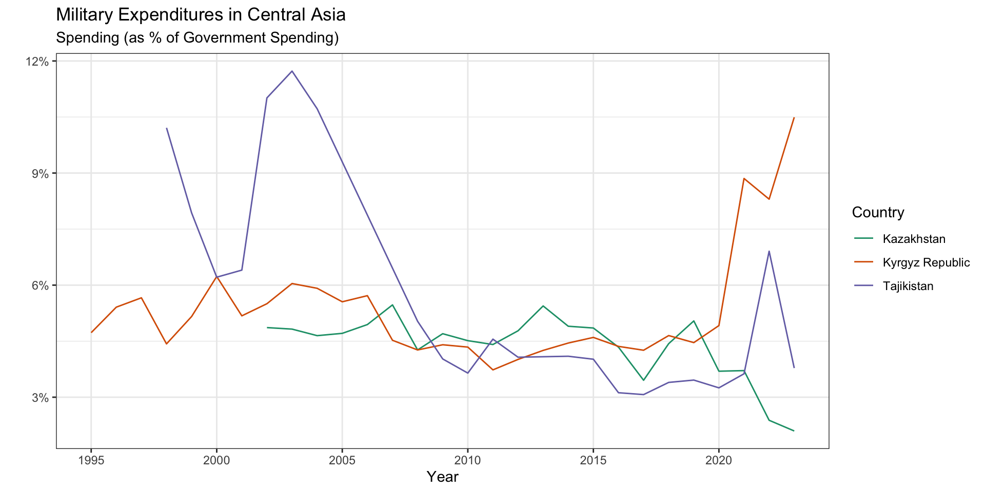

Inside ggplot(), we can order factor levels by the \(y\) values associated with the largest \(x\) values.

military_long |> 
  filter(Country %in% central.asia,
         !is.na(spending)) |> 
  ggplot(aes(x = year,
             y = spending,
             color = fct_reorder2(.x = year,
                                  .y = spending,
                                  .f = Country))) +
  geom_line() +
  labs(x = "Year",
       y = "",
       color = "Country",
       subtitle = "Spending (as % of Government Spending)",
       title = "Military Expenditures in Central Asia") +
  scale_color_manual(values = brewer.pal(3, "Dark2")) +
  scale_y_continuous(labels = scales::percent) +
  scale_x_continuous(breaks = seq(1990, 2023, 5)) +
  theme_bw() +
  theme(panel.grid.minor.x = element_blank())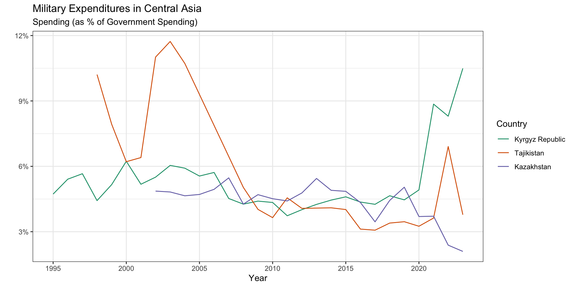

Why Mess with Factors?

Discussion

What are some of the benefits to re-ordering or re-leveling factors variables?

`janitor` Package

Variable Names in R

Data from external sources likely has variable names not ideally formatted for R.

Names may…

contain spaces.
start with numbers.
start with a mix of capital and lower case letters.

names(military)[1:12]

 [1] "Country"        "Notes"          "Reporting year" "1988.0"        
 [5] "1989.0"         "1990.0"         "1991.0"         "1992.0"        
 [9] "1993.0"         "1994.0"         "1995.0"         "1996.0"

Messy Variable Names are a Pain

You should have noticed this in Practice Activity 4 working with the SIPRI data
You have to use back tick marks around variables that start with numbers or have spaces:

military |> 
  select(`Reporting year`,
          `1988.0`)

I personally find capitilization in variable names is very annoying and slows me down

`janitor` to the rescue!

Mr. Johnson from Abbot Elementary (https://giphy.com/abcnetwork)

Clean Variable Names with `janitor`

The janitor package converts all variable names in a dataset to snake_case.

Names will…

start with a lower case letter.
have spaces and special characters filled in with _.

library(janitor)
military_clean_names <- military |> 
  clean_names()

names(military_clean_names)[1:12]

 [1] "country"        "notes"          "reporting_year" "x1988_0"       
 [5] "x1989_0"        "x1990_0"        "x1991_0"        "x1992_0"       
 [9] "x1993_0"        "x1994_0"        "x1995_0"        "x1996_0"

Lifecycle Stages

`R` Is Always Evolving

Remember: R is open source so folks are always adding and updating packages and functions

Discussion

What benefits and drawbacks of R’s ever-evolving nature have you noticed?

the good 🥳
the annoying

always (aiming) to get better!
responsive to user input
new functionality for new statistical methods

code may no longer run after an update 😭
need to learn new syntax
have to keep track of it all 🫠

Lifceycle Stages

As packages get updated, the functions and function arguments included in those packages will change.

The accepted syntax for a function may change.
A function/functionality may disappear.

Learn more about lifecycle stages of packages, functions, function arguments in R.

Lifceycle Stages

Deprecated Functions

A deprecated functionality has a better alternative available and is scheduled for removal.

You get a warning telling you what to use instead.

military_clean |> 
  filter(across(!Country, is.na)) |> 
  slice_head(n = 3) |> 
  select(1:8)

Warning: Using `across()` in `filter()` was deprecated in dplyr 1.0.8.
ℹ Please use `if_any()` or `if_all()` instead.

# A tibble: 3 × 8
  Country         `1988.0` `1989.0` `1990.0` `1991.0` `1992.0` `1993.0` `1994.0`
  <chr>           <chr>    <chr>    <chr>    <chr>    <chr>    <chr>    <chr>   
1 Africa          <NA>     <NA>     <NA>     <NA>     <NA>     <NA>     <NA>    
2 North Africa    <NA>     <NA>     <NA>     <NA>     <NA>     <NA>     <NA>    
3 sub-Saharan Af… <NA>     <NA>     <NA>     <NA>     <NA>     <NA>     <NA>

Deprecated Functions

You should not use deprecated functions!

Instead, we use…

military_clean |>
  filter(if_all(!Country, ~ is.na(.x))) |> 
  slice_head(n = 3) |> 
  select(1:8)

# A tibble: 3 × 8
  Country         `1988.0` `1989.0` `1990.0` `1991.0` `1992.0` `1993.0` `1994.0`
  <chr>           <chr>    <chr>    <chr>    <chr>    <chr>    <chr>    <chr>   
1 Africa          <NA>     <NA>     <NA>     <NA>     <NA>     <NA>     <NA>    
2 North Africa    <NA>     <NA>     <NA>     <NA>     <NA>     <NA>     <NA>    
3 sub-Saharan Af… <NA>     <NA>     <NA>     <NA>     <NA>     <NA>     <NA>

Superceded Functions

A superseded functionality has a better alternative, but is not going away.

This is a softer alternative to deprecation.
A superseded function will not give a warning (since there’s no risk if you keep using it), but the documentation will give you a recommendation.

Lab 4: Childcare Costs in California

To do…

Lab 4: Childcare Costs in California
- Due Monday 4/28 at 11:59pm
Read Chapter 5: Strings + Dates
- Check-in 5.1 - 5.2 due Tuesday (4/29) before class

Extending Data Joins + Factors

Thursday, April 24

Project

Extensions to Relational Data

Relational Data Reminder - Keys

IMDb Movies Data

Joining Multiple Data Sets

Know Your Unique Observations!

Know Your Unique Observations!

Know Your Unique Observations!

Joining on Multiple Variables

Factor Variables

What is a factor variable?

Eras Tour

Creating a Factor – Base R

Creating a Factor – Base R

Creating a Factor – Base R

forcats

Creating a Factor – fct

Creating a Factor – fct

Creating a Factor – fct

Re-coding a Factor – fct_recode

Re-coding a Factor – case_when

Collapsing a Factor –fct_collapse

Re-leveling a Factor –fct_relevel

Re-ordering Factors in ggplot2

Re-ordering Factors in ggplot2

Re-ordering Factors in ggplot2

Re-ordering Factors in ggplot2

Why Mess with Factors?

janitor Package

Variable Names in R

Messy Variable Names are a Pain

janitor to the rescue!

Clean Variable Names with janitor

Lifecycle Stages

R Is Always Evolving

Lifceycle Stages

Lifceycle Stages

Deprecated Functions

Deprecated Functions

Superceded Functions

Lab 4: Childcare Costs in California

To do…

Creating a Factor – Base `R`

Creating a Factor – Base `R`

Creating a Factor – Base `R`

`forcats`

Creating a Factor – `fct`

Creating a Factor – `fct`

Creating a Factor – `fct`

Re-coding a Factor – `fct_recode`

Re-coding a Factor – `case_when`

Collapsing a Factor –`fct_collapse`

Re-leveling a Factor –`fct_relevel`

Re-ordering Factors in `ggplot2`

Re-ordering Factors in `ggplot2`

Re-ordering Factors in `ggplot2`

Re-ordering Factors in `ggplot2`

`janitor` Package

`janitor` to the rescue!

Clean Variable Names with `janitor`

`R` Is Always Evolving